Chapter 16 Stratification
Stratification occurs when we are sampling units in the population of interest within some prespecified categories. The main goal of stratification is to ensure that the surveyed sample reflects as much as possible the composition of the original population, at least in terms of the categories used to stratify. In randomized experiments, stratification is used to ensure that the control and treatment groups are as similar as possible. At least in theory, stratification helps to improve precision, since it decreases the amount of variation in the unobserved confounders that might not be aligned between treatment and control groups and that are the cause of sampling noise. Stratification is thus a very powerful tool to improve the precision of treatment effect estimates, without having to increase sample size.
There are several key issues around stratification. The first is how to implement it in practice. One key issue is which covariates to choose and how to combine them in order not to end up with too many small cells. A second key issue is how to estimate sampling noise after stratification. An easy mistake is to stratify and then forget about stratification when estimating sampling noise, thereby inflating sampling noise, and missing the improvements brought about by the stratification process.
One solution to these issues that I particularly like is to conduct a pairwise RCT, that is to have strata of size two. The main advantage of this solution is that it theoretically solves the problem of combining covariates optimally: just find the pairs of observations that look most alike and randomize the treatment between them. One difficulty with this approach is that finding the pairs that minimize the overall distance between them is a difficult task. Until now, it was solved using undirected search algorithms which simply go through all the possible combinations to try to find the optimal one. This poses two problems: the pairing you find is not ensured to be the best one and finding it might take a lot of time. In this chapter, I introduce a pairing algorithm that finds the optimal pairs in polynomial (e.g. reasonable) time.
Another approach would be to generate the strata by k-means clustering. Intuitively, the pairwise RCT approach should minimize residual errors, but a formal proof of that result does not exist. A full treatment of optimal stratification is still missing, at least to my knowledge, in the literature.
I am going to first examine the analysis of classical stratified experiments (with more than 2 units per strata) first, then I’ll turn to pairwise RCTs and finally I’ll examine how you stratify in practice.
16.1 Analysis of classical stratified experiments
We are first going to look at an example to see how stratification can help with sampling noise, basically decreasing it by a starkly large factor. We will then study the estimation of treatment effects under stratified randomization and then the estimation of sampling noise, which is a critical phase in order for our precision estimates to reflect the increase in precision brought about by stratification.
16.1.1 An example
Let us first generate a stratified random sample in order to see what stratification can do for us, and what a naive approach to the analysis of stratified experiments misses. We are going to study the case of a Brute Forced design, and we will vary the amount of stratification, from none to a lot of strata. In practice, there are several ways to build strata and to draw observations within each of them. Here, I am only going to stratify on one pre-treatment variable, pre-treatment outcome. But, in practice, stratification is done on several variables that we need to interact. One way to build groups with similar values of these variables is to use \(k\)-means clustering. \(k\)-means clustering finds the optimal separation of points in the sample between a pre-specified number of \(k\) clusters such that the within-cluster variance is minimized (so that the strata (i.e. clusters) are as homogeneous as possible, which is our goal when stratifying among similar units of observations). Whether using \(k\)-means clustering, or simply by selecting sets of observations which have similar values for their covariates, we end up with a set \(\mathcal{S}\) of strata.
Once the strata are built, there are several ways to select the treated units within each strata. Section 3 in Bugny, Canay and shaikh (2018) gives several examples of stratified assignments. The one we are going to use here is stratified block randomization. In this approach we select, in each strata \(s\in\mathcal{S}\) of size \(N_s\), a number \(N^1_s\) of observations for receiving the treatment, with \(N^1_s=\lfloor \pi N_s \rfloor\), with \(\pi\) the target proportion of treated and control units in the sample.
Remark. Note that with stratified block randomization and \(\pi\) constant with \(s\), each strata will be represented in the sample in proportion to its weight in the population. Other designs have \(\pi\) vary with \(s\), but we are not going to examine them here. See Imbens and Rubin (2015) for more details on how to analyze them.
Remark. Another point worthy of notice is that stratified block randomization is not what we have used when we have drawn random samples for RCTs in Chapter 3. In that chapter, we have used a simple coin design, in which each unit is affected either to the treatment or to the control as a function of an independent coin toss. As a result, the actual proportion of of treated and control in the sample is not exactly \(\pi\). But the Law of Large Numbers ensures that the actual proportion is not very far from the target \(\pi\). Since strata are small, the Law of Large Number does not apply as fast, and imbalances might arise in pratice because of variations in the proportion of treated units across strata. Hence, we prefer to use stratified block randomization.
Example 16.1 Let’s see how this works in our ususal example of a brute force design, with stratification on the pre-treatment outcomes \(y^B_i\).
Let us first generate a random sample.
param <- c(8,.5,.28,1500,0.9,0.01,0.05,0.05,0.05,0.1)
names(param) <- c("barmu","sigma2mu","sigma2U","barY","rho","theta","sigma2epsilon","sigma2eta","delta","baralpha")set.seed(1234)
N <-1000
mu <- rnorm(N,param["barmu"],sqrt(param["sigma2mu"]))
UB <- rnorm(N,0,sqrt(param["sigma2U"]))
yB <- mu + UB
YB <- exp(yB)
epsilon <- rnorm(N,0,sqrt(param["sigma2epsilon"]))
eta<- rnorm(N,0,sqrt(param["sigma2eta"]))
U0 <- param["rho"]*UB + epsilon
y0 <- mu + U0 + param["delta"]
alpha <- param["baralpha"]+ param["theta"]*mu + eta
y1 <- y0+alpha
Y0 <- exp(y0)
Y1 <- exp(y1)
data.strata <- data.frame(yB=yB,y1=y1,y0=y0) %>%
mutate(
id = 1:N
)Let us now generate several sets of strata using \(k\)-means clustering, with the command stats::kmeans.
We are going to vary the number of strata, from \(1\) to \(100\).
# function generating $k$ strata based on a dataset of pre-treatment variables using k-means clustering
# k: number of strata
# data: the dataset used for stratification
# var: the list of variables used for stratification
stratification <- function(k,var,data){
  data.strat <- data %>%
                  select(contains(var))
  k.means <- stats::kmeans(data.strat,centers=k,nstart=k)
  strata.k <- as.data.frame(k.means$cluster)
  colnames(strata.k) <- c(paste("strata",k,sep='_'))
  return(strata.k)
}
# test
strata.2 <- stratification(k=2,var="yB",data=data.strata)
strata.5 <- stratification(k=5,var="yB",data=data.strata)
#data <- cbind(data,strata=strata.2$cluster)
# let us now map across values of $k$
k.vec <- c(1,2,5,10,25,50,100)
test.map <- map(k.vec,stratification,var="yB",data=data.strata) %>%
              bind_cols()
# final data
data.strata <- cbind(data.strata,test.map)
# counting strata size
#strata.size <- data.strata %>%
Let us finally visualize the grouping with 5 and 50 strata.
ggplot(data.strata,aes(x=yB,y=y0,group=as.factor(strata_5),color=as.factor(strata_5),shape=as.factor(strata_5)))+
  geom_point()+
  theme_bw()

ggplot(data.strata,aes(x=yB,y=y0,group=as.factor(strata_50),color=as.factor(strata_50)))+
  geom_point()+
  theme_bw()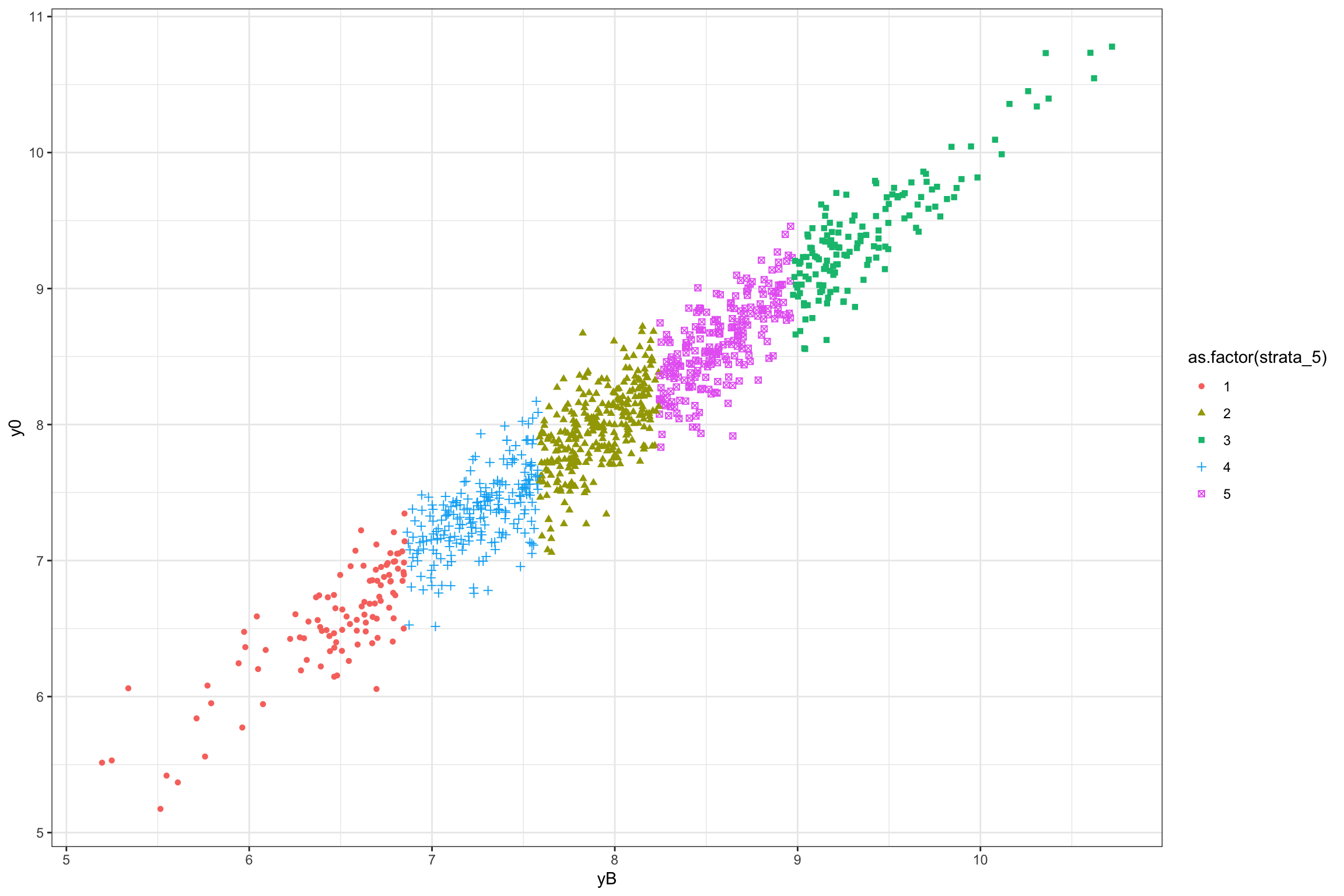
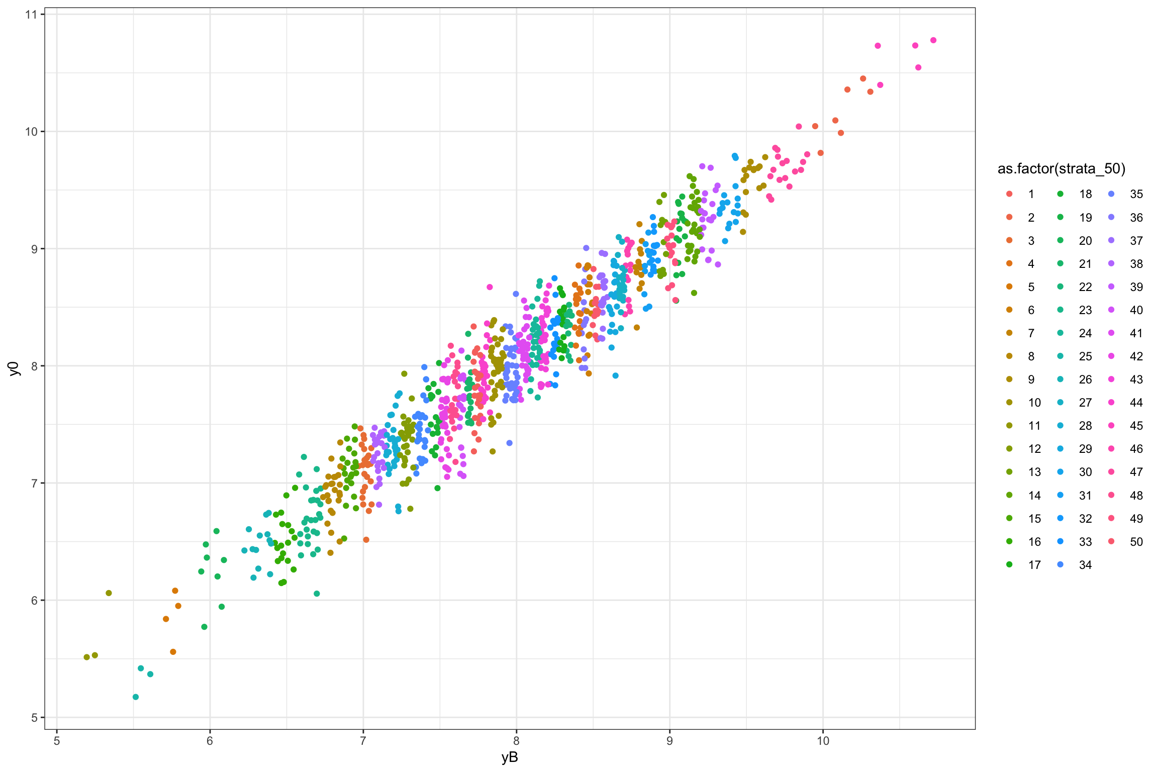
Figure 16.1: Grouping in strata using \(k\)-means clustering
Each strata is defined as an upper and lower bound on the value of \(y_i^B\), so as to be mutually exclusive. The effectiveness of the strata at increasing precision and power stems from the fact that \(y_i^B\) is strongly correlated with \(y_i^0\), thereby decreasing the likelihood that treated and control units have different distributions of potential outcomes. Because of that property, we would like the number of strata to be as big as possible. But this generates one problem: we might end up with strata that only have one unit. In that case, we cannot randomly allocate the treatment within the strata, and we have to exclude it from our sample, thereby losing its representativity. This problem is even more serious if we have several treatments that we want to test against our control. As a consequence, we cannot increase the number of strata indefinitely. Let’s see how the strata are composed in our example.
StrataSize <- data.strata %>%
                pivot_longer(cols=contains('strata'),names_to = "strata_type",values_to="strata_value") %>%
                group_by(strata_type,strata_value) %>%
                summarise(
                  Ns = n()
                ) %>%
                  mutate(
                  strata_N = str_split_fixed(strata_type,'_',2)[,2],
                  strata_N = factor(strata_N,levels=c('1','2','5','10','25','50','100')),
                  strata_value = as.factor(strata_value)
                )

StrataSizeMinMedMax <- StrataSize %>%
                group_by(strata_type,strata_N) %>%
                summarise(
                  Min = min(Ns),
                  Max = max(Ns),
                  Mean = mean(Ns)
                ) %>%
                pivot_longer(cols= Min:Mean,names_to = "Type",values_to = "Stat") %>%
                mutate(
                  Type = factor(Type,levels=c('Min','Mean','Max'))
                )
Let us plot the resulting minimum value of strata size:
ggplot(StrataSize %>% filter(strata_N!='1'),aes(x=strata_value,y=Ns,fill=strata_value)) +
    geom_bar(stat='identity') +
    geom_hline(aes(yintercept=1),color='red',linetype='dotted') +
    #scale_y_continuous(trans=log_trans(),breaks=c(1,10,100))+
    #expand_limits(y=0) +
    scale_fill_discrete(name='Strata') +
    xlab('Strata')+
    ylab('Strata size')+
    theme_bw() +
    facet_grid(strata_N~.)

ggplot(StrataSizeMinMedMax,aes(x=strata_N,y=Stat,fill=Type,group=Type)) +
    geom_bar(stat='identity',position=position_dodge()) +
    geom_hline(aes(yintercept=1),color='red',linetype='dotted') +
    #scale_y_continuous(trans=log_trans(),breaks=c(1,10,100))+
    #expand_limits(y=0) +
    #scale_fill_discrete(name='Strata') +
    xlab('Number of strata')+
    ylab('Strata size')+
    theme_bw() #+
    #facet_grid(Type~.)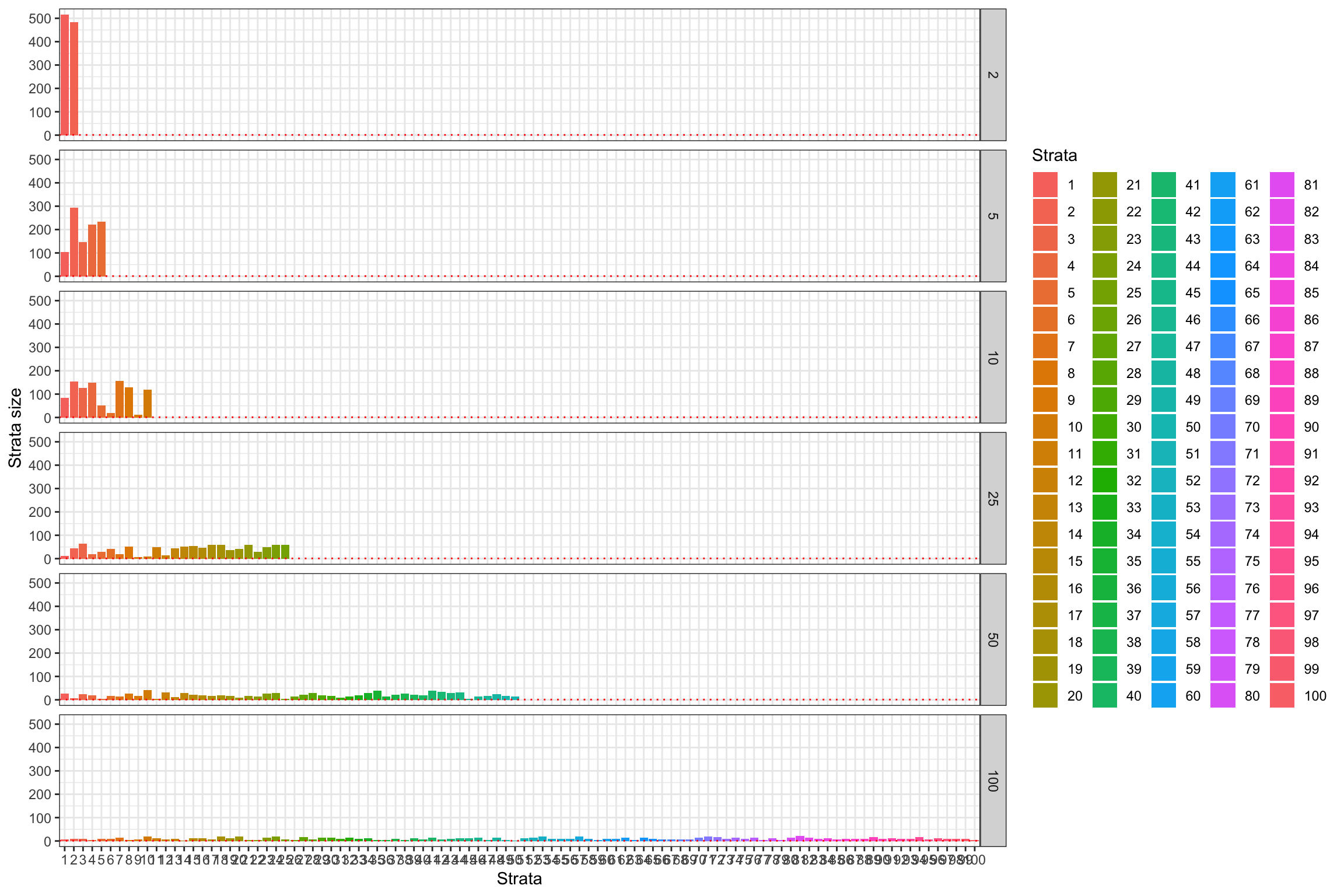
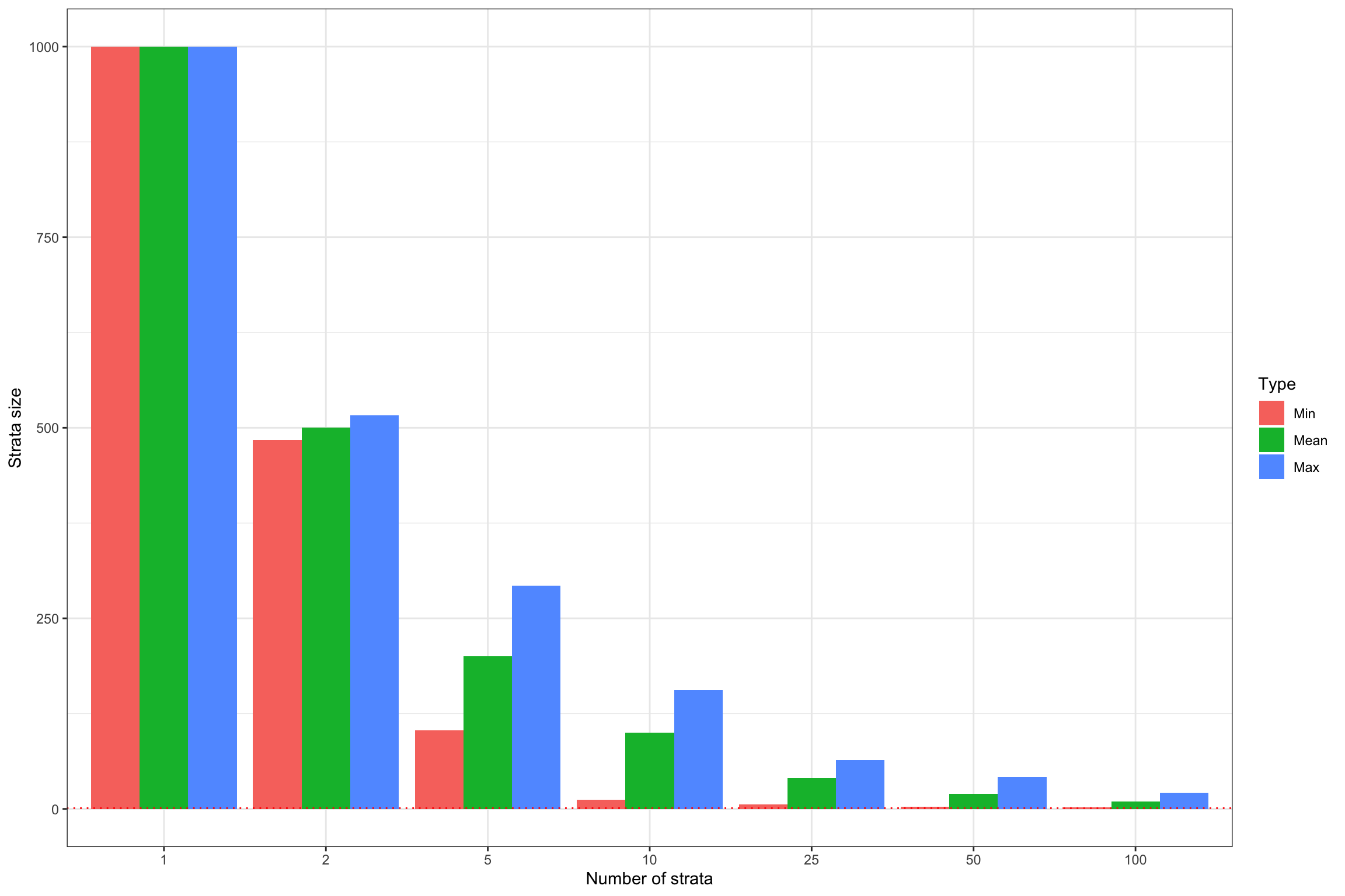
Figure 16.2: Number of strata and strata size
Let us now randomly allocate the treatment among strata using block randomization. The way I am going to do that is by randomly allocating a uniform random variable, compute its median in each strata and allocate everyone strictly below the median to the treatment, and everyone equal or above to the control. Let’s see how this works.
# number of strata types
NStrataTypes <- data.strata %>% select(contains('strata')) %>% colnames(.) %>% length(.)
set.seed(1234)
data.strata <- data.strata %>%
                pivot_longer(cols=contains('strata'),names_to = "strata_type",values_to="strata_value") %>%
                mutate(
                  strata_type_value = str_c(strata_type,strata_value,sep='_'),
                  strata_value = as.factor(strata_value),
                  strata_type = as.factor(strata_type)
                ) %>%
                mutate(
                  randU = runif(N*NStrataTypes)
                ) %>%
                group_by(strata_type_value) %>%
                mutate(
                  randUMedStrata = stats::median(randU),
                  Ds = case_when(
                    randU<randUMedStrata ~ 1,
                    TRUE ~ 0
                  ),
                  y = y1*Ds+(1-Ds)*y0,
                  Ns = n(),
                  pis = mean(Ds)
                ) %>%
                arrange(strata_type,Ns,strata_value,randU)
Let us now examine how to estimate the treatment effect in this sample. One key question here is how to compute the treatment effect estimate. There are at least four different ways:
- Use the simple with/without estimator.
- Use a weighted average of the treatment effects in each strata, with weights proportionnal to the inverse of their variance.
- Use an OLS regression with the treatment dummy and a set of strata fixed effects.
- Use an OLS regression with the treatment dummy and a set of strata fixed effects interacted with the treatment indicator (this is a fully saturated model).
We will examine later the rationale for each of these estimators. For now, I am going to compute the distribution of the simple with/without estimator and of the strata fixed effects estimator.
# WW
regWW <- data.strata %>%
        group_by(strata_type) %>%
        nest(.) %>%
       # rowwise(.) %>%
        mutate(
          reg = map(data,~lm(y~Ds,data=.)),
          tidied = map(reg,tidy)
        ) %>%
        unnest(tidied) %>%
        filter(term == 'Ds') %>%
        rename(
          Coef = estimate,
          Se = std.error
        ) %>%
        select(strata_type,Coef,Se)%>%
        mutate(Type='WW')
# strata fixed effects
regSFE <- data.strata %>%
        filter(strata_type!='strata_1') %>%
        group_by(strata_type) %>%
        nest(.) %>%
       # rowwise(.) %>%
        mutate(
          reg = map(data,~feols(y~Ds|strata_value,vcov="HC1",data=.)),
          tidied = map(reg,tidy)
        ) %>%
        unnest(tidied) %>%
        filter(term == 'Ds') %>%
        rename(
          Coef = estimate,
          Se = std.error
        ) %>%
        select(strata_type,Coef,Se) %>%
        mutate(Type='SFE')

# fully staturated model
# run a regression in each strata
regSAT <- data.strata %>%
#          filter(strata_type!='strata_1') %>%
          group_by(strata_type_value) %>%
          # generating the number of treated observations in each strata
          # and the proportion of observations in each strata
          mutate(
            Ns1 = sum(Ds),
            qs = Ns/N
          ) %>%
        filter(Ns1>1,N-Ns1>1) %>%
        nest(.) %>%
       # rowwise(.) %>%
        mutate(
          reg = map(data,~feols(y~Ds|1,vcov="HC1",data=.)),
          tidied = map(reg,tidy)
        ) %>%
        unnest(tidied) %>%
        filter(term == 'Ds') %>%
        rename(
          Coef = estimate,
          Se = std.error
        ) %>%
        select(strata_type_value,Coef,Se)

# weighted mean function over a dataset with a formula for use in nest
# formula: formula with outcome as regressand and weigths as regressors
# data: the dataset used
weighted.mean.nest <- function(form,data,...){
  name.y <- as.character(form[[2]])
  name.w <- as.character(form[[3]])
  w.mean <- weighted.mean(x=data[name.y],w=data[name.w],...)
  return(w.mean)
}
# testing
test.wmean <- weighted.mean.nest(Coef~Se,data=regSAT,na.rm=TRUE)

# averaging back using strata proportions
regSAT.inter <- data.strata %>%
                group_by(strata_type,strata_value,strata_type_value) %>%
                summarize(
                  qs = mean(Ns/N),
                  Ns=mean(Ns),
                  Ns1 = sum(Ds)
                ) %>%
                # joigning with regression estimates
                left_join(regSAT,by='strata_type_value') %>%
                # creating variance terms
                mutate(
                  Var = Ns*Se^2
                ) %>%
                group_by(strata_type) %>%
                nest(.) %>%
                mutate(
                  Coef = map_dbl(data,~weighted.mean.nest(Coef~qs,data=.,na.rm=TRUE)),
                  Var = map_dbl(data,~weighted.mean.nest(Var~qs,data=.,na.rm=TRUE))
                ) %>%
                mutate(
                  Se = sqrt(Var/N)
                ) %>%
                select(strata_type,Coef,Se) %>%
                mutate(Type='SAT')

# Bugni, Canay and Shaikh correction (adding VH)
regSAT.BCS <- data.strata %>%
                group_by(strata_type,strata_value,strata_type_value) %>%
                summarize(
                  qs = mean(Ns/N),
                  Ns=mean(Ns),
                  Ns1 = sum(Ds)
                ) %>%
                # joigning with regression estimates
                left_join(regSAT,by='strata_type_value') %>%
                select(contains('strata'),qs,Coef) %>%
                rename(WW=Coef) %>%
                left_join(regWW,by='strata_type') %>%
                select(contains('strata'),qs,Coef,WW) %>%
                mutate(
                  diffCoefSq = (Coef-WW)^2
                ) %>%
                group_by(strata_type) %>%
                nest(.) %>%
                mutate(
                  VH = map_dbl(data,~weighted.mean.nest(diffCoefSq~qs,data=.,na.rm=TRUE))
                ) %>%
                select(-data) %>%
                left_join(regSAT.inter,by='strata_type') %>%
                mutate(
                  Se = sqrt(Se^2+VH/N),
                  Type = "SAT.BCS"
                ) %>%
                select(-VH)

# regrouping
reg <- rbind(regWW,regSFE,regSAT.inter,regSAT.BCS)
Let us now write a function to parallelize these simulations.
# function generating one set of simulated estimates of the WW and SFE estimator under stratification
# s: random seed
# N: sample size
# Nstrata: number of strata (can be a vector)
# param: parameter to generate sample
monte.carlo.brute.force.ww.yB.strata <- function(s,N,Nstrata,param){
  # generating random sample
  set.seed(s)
  mu <- rnorm(N,param["barmu"],sqrt(param["sigma2mu"]))
  UB <- rnorm(N,0,sqrt(param["sigma2U"]))
  yB <- mu + UB
  YB <- exp(yB)
  epsilon <- rnorm(N,0,sqrt(param["sigma2epsilon"]))
  eta<- rnorm(N,0,sqrt(param["sigma2eta"]))
  U0 <- param["rho"]*UB + epsilon
  y0 <- mu +  U0 + param["delta"]
  alpha <- param["baralpha"]+  param["theta"]*mu + eta
  y1 <- y0+alpha
  Y0 <- exp(y0)
  Y1 <- exp(y1)
  data.strata <- data.frame(yB=yB,y1=y1,y0=y0) %>%
                  mutate(
                    id = 1:N
                  )
  # generating strata
  strata <- map(Nstrata,stratification,var="yB",data=data.strata) %>%
              bind_cols()
  data.strata <- cbind(data.strata,strata)
  # allocating the treatment
  # number of strata types
  NStrataTypes <- data.strata %>% select(contains('strata')) %>% colnames(.) %>% length(.)
  set.seed(s)
  data.strata <- data.strata %>%
                  pivot_longer(cols=contains('strata'),names_to = "strata_type",values_to="strata_value") %>%
                  mutate(
                    strata_type_value = str_c(strata_type,strata_value,sep='_'),
                    strata_value = as.factor(strata_value),
                    strata_type = as.factor(strata_type)
                  ) %>%
                  mutate(
                    randU = runif(N*NStrataTypes)
                  ) %>%
                  group_by(strata_type_value) %>%
                  mutate(
                    randUMedStrata = stats::median(randU),
                    Ds = case_when(
                      randU<randUMedStrata ~ 1,
                      TRUE ~ 0
                    ),
                    y = y1*Ds+(1-Ds)*y0,
                    Ns = n(),
                    pis = mean(Ds)
                  ) %>%
                  arrange(strata_type,Ns,strata_value,randU)
  # estimating the treatment effects
  # WW
  regWW <- data.strata %>%
          group_by(strata_type) %>%
          nest(.) %>%
         # rowwise(.) %>%
          mutate(
            reg = map(data,~feols(y~Ds|1,vcov="HC1",data=.)),
            tidied = map(reg,tidy)
          ) %>%
          unnest(tidied) %>%
          filter(term == 'Ds') %>%
          rename(
            Coef = estimate,
            Se = std.error
          ) %>%
          select(strata_type,Coef,Se)%>%
          mutate(Type='WW')
  # strata fixed effects
  regSFE <- data.strata %>%
          filter(strata_type!='strata_1') %>%
          group_by(strata_type) %>%
          nest(.) %>%
         # rowwise(.) %>%
          mutate(
            reg = map(data,~feols(y~Ds|strata_value,vcov="HC1",data=.)),
            tidied = map(reg,tidy)
          ) %>%
          unnest(tidied) %>%
          filter(term == 'Ds') %>%
          rename(
            Coef = estimate,
            Se = std.error
          ) %>%
          select(strata_type,Coef,Se) %>%
          mutate(Type='SFE')

  # fully staturated model
  # run a regression in each strata
  regSAT <- data.strata %>%
  #          filter(strata_type!='strata_1') %>%
            group_by(strata_type_value) %>%
            # generating the number of treated observations in each strata
            # and the proportion of observations in each strata
            mutate(
              Ns1 = sum(Ds),
              qs = Ns/N
            ) %>%
          filter(Ns1>1,N-Ns1>1) %>%
          nest(.) %>%
         # rowwise(.) %>%
          mutate(
           reg = map(data,~feols(y~Ds|1,vcov="HC1",data=.)),
           tidied = map(reg,tidy)
          ) %>%
          unnest(tidied) %>%
          filter(term == 'Ds') %>%
          rename(
            Coef = estimate,
            Se = std.error
          ) %>%
          select(strata_type_value,Coef,Se)

  # averaging back using strata proportions
  regSAT.inter <- data.strata %>%
                  group_by(strata_type,strata_value,strata_type_value) %>%
                  summarize(
                    qs = mean(Ns/N),
                    Ns=mean(Ns),
                    Ns1 = sum(Ds)
                  ) %>%
                  # joigning with regression estimates
                  left_join(regSAT,by='strata_type_value') %>%
                  # creating variance
                  mutate(
                    Var = Se^2*Ns
                  ) %>%
                  group_by(strata_type) %>%
                  nest(.) %>%
                  mutate(
                    Coef = map_dbl(data,~weighted.mean.nest(Coef~qs,data=.,na.rm=TRUE)),
                    Var = map_dbl(data,~weighted.mean.nest(Var~qs,data=.,na.rm=TRUE))
                  ) %>%
                  mutate(
                    Se = sqrt(Var/N)
                  ) %>%
                  select(strata_type,Coef,Se) %>%
                  mutate(Type='SAT')

  # Bugni, Canay and Shaikh correction (adding VH)
  regSAT.BCS <- data.strata %>%
                group_by(strata_type,strata_value,strata_type_value) %>%
                summarize(
                  qs = mean(Ns/N),
                  Ns=mean(Ns),
                  Ns1 = sum(Ds)
                ) %>%
                # joigning with regression estimates
                left_join(regSAT,by='strata_type_value') %>%
                select(contains('strata'),qs,Coef) %>%
                rename(WW=Coef) %>%
                left_join(regWW,by='strata_type') %>%
                select(contains('strata'),qs,Coef,WW) %>%
                mutate(
                  diffCoefSq = (Coef-WW)^2
                ) %>%
                group_by(strata_type) %>%
                nest(.) %>%
                mutate(
                  VH = map_dbl(data,~weighted.mean.nest(diffCoefSq~qs,data=.,na.rm=TRUE))
                ) %>%
                select(-data) %>%
                left_join(regSAT.inter,by='strata_type') %>%
                mutate(
                  Se = sqrt(Se^2+VH/N),
                  Type = "SAT.BCS"
                ) %>%
                select(-VH)

  # regrouping
  reg <- rbind(regWW,regSFE,regSAT.inter,regSAT.BCS)
  # adding the SFE estimator for strata 1
  regStrata1 <- reg %>%
                filter(strata_type=='strata_1') %>%
                mutate(
                  Type="SFE"
                )
  reg <- rbind(reg,regStrata1) %>%
         mutate(
           IdSim=s
         )
  return(reg)
}

simuls.brute.force.ww.yB.N.strata <- function(N,Nsim,Nstrata,param){
#  simuls.brute.force.ww.yB.N.strata <- as.data.frame(matrix(unlist(lapply(1:Nsim,monte.carlo.brute.force.ww.yB.strata,N=N,param=param,Nstrata=Nstrata)),nrow=2*length(Nstrata)*Nsim,ncol=5,byrow=TRUE))
  simuls.brute.force.ww.yB.N.strata <- lapply(1:Nsim,monte.carlo.brute.force.ww.yB.strata,N=N,param=param,Nstrata=Nstrata) %>%
                                        bind_rows(.)
#  colnames(simuls.brute.force.ww.yB.N.strata) <- c('strata_type','Coef','Se','Type','IdSim')
  return(simuls.brute.force.ww.yB.N.strata)
}

sf.simuls.brute.force.ww.yB.N.strata <- function(N,Nsim,Nstrata,param,ncpus){
  sfInit(parallel=TRUE,cpus=ncpus)
  sfExport('stratification')
  sfExport('weighted.mean.nest')
  sfLibrary(tidyverse)
  sfLibrary(stats)
  sfLibrary(fixest)
  sfLibrary(broom)
#  sim <- as.data.frame(matrix(unlist(sfLapply(1:Nsim,monte.carlo.brute.force.ww.yB.strata,N=N,param=param,Nstrata=Nstrata)),nrow=2*length(Nstrata)*Nsim,ncol=5,byrow=TRUE))
  sim <- sfLapply(1:Nsim,monte.carlo.brute.force.ww.yB.strata,N=N,param=param,Nstrata=Nstrata) %>%
         bind_rows(.)
  sfStop()
  return(sim)
}

Nsim <- 1000
#Nsim <- 10
#N.sample <- c(100,1000,10000,100000)
#N.sample <- c(100,1000,10000)
#N.sample <- c(100,1000)
N.sample <- c(1000)

Nstrata <- k.vec
#test <- simuls.brute.force.ww.yB.N.strata(N=N.sample,Nsim=Nsim,Nstrata=Nstrata,param=param)
simuls.brute.force.ww.yB.strata <- lapply(N.sample,sf.simuls.brute.force.ww.yB.N.strata,Nsim=Nsim,Nstrata=Nstrata,param=param,ncpus=2*ncpus)
## Library tidyverse loaded.
## Library stats loaded.
## Library fixest loaded.
## Library broom loaded.Let us now check the results.
SummaryStrata <- simuls.brute.force.ww.yB.strata[[1]] %>%
                  group_by(strata_type,Type) %>%
                  summarize(
                    MeanCoef = mean(Coef,na.rm=TRUE),
                    SdCoef = sd(Coef,na.rm=TRUE),
                    MeanSe = mean(Se,na.rm=TRUE)
                  ) %>%
                  mutate(
                    strata_size = str_split_fixed(strata_type,'\\_',n=2)[,2],
                    strata_size = factor(strata_size,levels=k.vec),
                    strata_type = factor(strata_type,levels=paste('strata',k.vec,sep='_')),
                    ATE = delta.y.ate(param),
                    Type = factor(Type,levels=c('WW','SFE','SAT','SAT.BCS'))
)ggplot(SummaryStrata %>% filter(Type!='SAT.BCS'),aes(x=strata_size,y=MeanCoef,color=Type,shape=Type))+
#geom_histogram(binwidth=.01, alpha=0.5,position='identity') +
#geom_density(alpha=0.3)+
#geom_bar(stat='identity',position=position_dodge())+
geom_pointrange(aes(ymin=MeanCoef-1.96*SdCoef,ymax=MeanCoef+1.96*SdCoef,color=Type,shape=Type),position=position_dodge(0.2))+
geom_hline(aes(yintercept=ATE),color='red',linetype='dotted') +
expand_limits(y=0)+
xlab('Number of strata')+
theme_bw()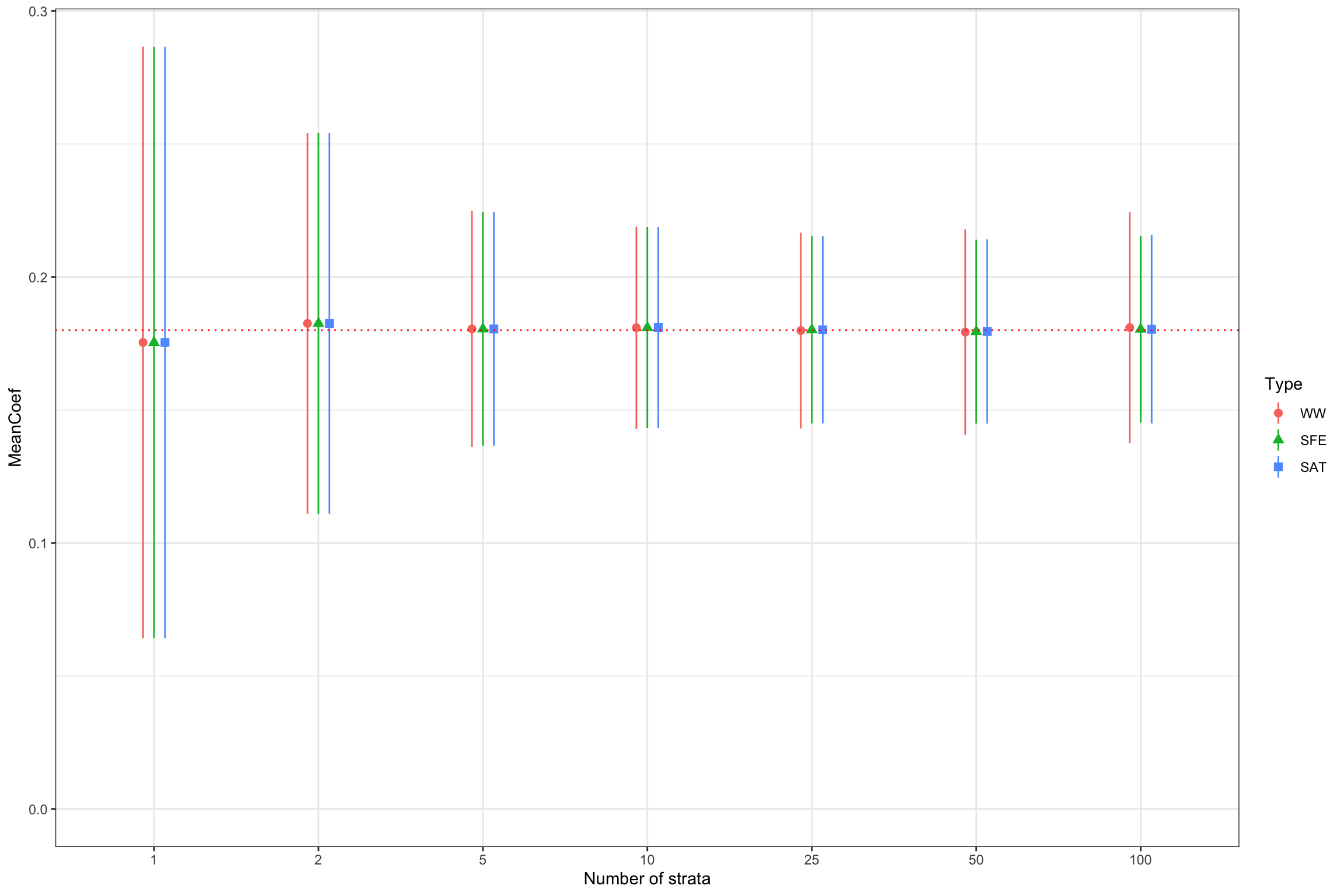
Figure 16.3: Distribution of estimators under various levels of stratification
Figure 16.3 clearly shows that stratification can increase precision. For the \(WW\) estimator, 99% sampling noise moves from 0.29 with one strata to 0.1 with 50 strata.
16.1.2 Estimating treatment effects with stratified randomized controlled trials
There are several ways to estimate average treatment effects under stratification. We have seen two un our example: the simple \(WW\) estimator and the strata fixed effects estimator. We are going to see that we could also use a fully saturated model, that in general, is not necessary, except when the target proportion of treated individuals changes with strata. Finally, we will study the precision weighted estimator, which is an instance of a meta-analytic estimator.
16.1.2.1 Using the \(WW\) estimator
The \(WW\) estimator simply compares the mean outcome of the treated and untreated individuals. As we have already seen in Chapter 3, this estimator can be computed using a simple OLS regression. We know thanks to Theorem 3.1 that the \(WW\) estimator is consistent under randomization, whatever the randomization device.
Remark. There is confusion as to whether this estimator will reflect the increase in precision brought about by stratification. Figure 16.3 shows that it is indeed the case: the precision of the \(WW\) estimator increases with the number of strata (up to 25 to 50 strata at least). Intuitively, this makes sense since the sample on which the \(WW\) estimator is estimated is already balanced on the observed characteristics used for stratification, and therefore its distribution is less affected by imbalances in these observed factors.
Remark. A different question is whether the default estimators of sampling noise of the \(WW\) estimator reflect the true extent of sampling noise, and especially are able to reflect the increase in precision due to stratification. The answer is in general no, and we will study estimators of sampling noise in the next section.
16.1.2.2 Using the strata fixed effects estimator
The strata fixed effects estimator is defined as the OLS estimate of \(\beta^{SFE}\) in the following regression:
\[\begin{align*} Y_i & = \sum_{s\in\mathcal{S}}\alpha^{SFE}_s\uns{\mathbf{s}(i)=s}+\beta^{SFE}R_i + \epsilon^{SFE}_i, \end{align*}\]
where \(\mathbf{s}(i)\) associates to each observation \(i\) in the sample the strata \(s\) to which it belongs. Conversely, and for later uses, \(\mathcal{I}_s\) is the set of units that belong to strata \(s\).
What does \(\beta^{SFE}\) estimate? We can first show that it is a weighted average of strata-level \(WW\) comparisons. For that, we need a slightly stronger assumption as the usual full rank assumption we have been using to analyze RCTs:
Hypothesis 16.1 (Full rank within strata) We assume that there is at least one observation in each strata that receives the treatment and one observation that does not receive it: \[\begin{align*} \forall s \in \mathcal{S}, \exists i,j\in \mathcal{I}_s \text{ such that } & D_i=1 \& D_j=0. \end{align*}\]
Theorem 16.1 (Decomposing the strata fixed effects estimator) Under Assumption 16.1, the strata fixed effects estimator is a weighted average of strata-level \(WW\) estimators:
\[\begin{align*} \hat{\beta}^{SFE} & = \sum_{s\in\mathcal{S}}w^{SFE}_s\hat{\Delta}^Y_{WW_s}\\ \hat{\Delta}^Y_{WW_s} & =\frac{\sum_{i:\mathbf{s}(i)=s}R_iY_i}{\sum_{i:\mathbf{s}(i)=s}R_i}-\frac{\sum_{i:\mathbf{s}(i)=s}(1-R_i)Y_i}{1-\sum_{i:\mathbf{s}(i)=s}R_i}\\ w^{SFE}_s & = \frac{N_s\bar{R}_s(1-\bar{R}_s)}{\sum_{s\in\mathcal{S}}N_s\bar{R}_s(1-\bar{R}_s)} \end{align*}\]
with \(\bar{R}_s=\frac{1}{N_s}\sum_{i:\mathbf{s}(i)=s}R_i\) and \(N_s\) is the size of strata \(s\).
Proof. See in Appendix A.7.1.
In order to prove the consistency of the strata fixed effects estimator, we need to slightly alter the usual independence assumption so that it reflects the fact that randomization occurs within each strata:
Hypothesis 16.2 (Independence within strata) We assume that the allocation of the program is independent of potential outcomes within each strata: \[\begin{align*} R_i\Ind(Y_i^0,Y_i^1)|\mathbf{s}(i). \end{align*}\]
We can now prove the consistency of the strata fixed effects estimator:
Theorem 16.2 (Consistency of the strata fixed effects estimator) Under Assumptions 16.2, 3.2 and 16.1, the strata fixed effects estimator is a consistent estimator of the Average Treatment Effect:
\[\begin{align*} \plims\hat{\beta}^{SFE} & = \Delta^Y_{ATE}. \end{align*}\]
Proof. See in Appendix A.7.2.
Remark. Note that Theorem 16.2 does not prove that the strata fixed effects estimator is unbiased. I am very close to proving that using an approach similar to the one developed in the proof of Lemma A.1. One thing that makes me fail in completing the proof is that the weights \(w_s\) are not independent of each other, neither is the numerator and denominator of each of them (because they share one strata in the denominator). Assuming this away (because each strata is small relative to the others) enables to prove unbiasedness. I am not aware of a general proof of unbiasedness for the strata fixed effects estimator. Let me know if you can find one.
16.1.2.3 Using the fully saturated estimator
A natural approach, similar to the one we used with DID with staggered designs in Section 4.3.3, is to estimate a treatment effect within each strata, and then to take a weighted average of these estimates with the appropriate weights in order to recover an adequate average treatment effect. This approach is akin to estimating a fully saturated model, since each strata has its own separate set of intercept and slope. The way we implement this estimator is by estimating the following model by OLS:
\[\begin{align*} Y_i & = \sum_{s\in\mathcal{S}}\alpha^{SAT}_s\uns{\mathbf{s}(i)=s}+\sum_{s\in\mathcal{S}}\beta_s^{SAT}\uns{\mathbf{s}(i)=s}R_i + \epsilon^{SAT}_i, \end{align*}\]
and then to reaggregate the individual strata estimates using the proportion of the observations that lie in each strata:
\[\begin{align*} \Delta^Y_{SAT} & = \sum_{s\in\mathcal{S}}w^{SAT}_s\beta_s^{SAT}\\ w^{SAT}_s & = \frac{N_s}{N}. \end{align*}\]
We can prove the following result:
Theorem 16.3 (Unbiasedness and consistency of the fully saturated model) Under Assumptions 3.1, 3.2 and 16.1, the fully saturated model is an unbiased and consistent estimator of the Average Treatment Effect:
\[\begin{align*} \esp{\hat{\Delta}^{Y}_{SAT}} & = \Delta^Y_{ATE}\\ \plims\hat{\Delta}^{Y}_{SAT} & = \Delta^Y_{ATE}. \end{align*}\]
Proof. See in Appendix A.7.3.
Remark. Imbens and Rubin (2015) define the fully saturated model as follows:
\[\begin{align*} Y_i & = \sum_{s\in\mathcal{S}}\alpha^{SAT}_s\uns{\mathbf{s}(i)=s}+\sum_{s\in\mathcal{S}\setminus{S}}\gamma^{SAT}_sR_i\left(\uns{\mathbf{s}(i)=s}-\uns{\mathbf{s}(i)=S}\frac{N_s}{N_S}\right)\\ & \phantom{=} +\beta^{SAT}R_i\frac{\uns{\mathbf{s}(i)=S}}{\frac{N_S}{N}} + \epsilon^{SAT}_i. \end{align*}\]
Their Theorem 9.2 shows that this definition is numerically equivalent to that in Theorem 16.3. I prefer using the OLS estimator in each strata and then averaging rather than building the complex estimator that Imbens and Rubin use.
16.1.3 Estimating sampling noise in stratified randomized controlled trials
We now have consistent (and even sometimes unbiased) estimators of the average treatment effect in a stratified experiment. Can we now estimate the sampling noise around these estimators?
Remark. One especially important question is whether we can form estimates of sampling noise that reflect the fact that stratification decreases sampling noise (if the stratification variables are correlated with potential outcomes). For example, the usual CLT-based estimator that we derived in Theorem 2.5 does not take into account that some stratification occurred. It will give an estimate of sampling noise that is correct for the case of one unique strata, but it fail at delivering estimates reflecting the increases in precision that occur after stratification.
Remark. Note that stratification improvemes precision also for the simple WW estimator, as Figure 16.3 shows. This means that even if the simple OLS estimator is consistent for the average treatment effect, its standard error will not. In general, it will be too big, and therefore confidence intervals based on it will be too large, which is a shame. That is why using consistent estimators of sampling noise matters.
Remark. A second concern is whether the default (heteroskedasticity robust) standard errors of the strata fixed effects estimator (SFE) provides an accurate estimate of the sampling noise of that estimator. Imbens and Rubin (2015) argue that it is the case while Bugny, Canay and shaikh (2018) and Bugny, Canay and shaikh (2019) disagree. As Bugny, Canay and shaikh (2019) explain in their Remark 5.1, the main difference between their approaches is whether you assume that your sampling scheme can be characterized by \(\frac{N_s}{N}\) being constant with \(N\). One way in which this might be true is that, each time we draw a new sample, we do not increase the number strata with sample size, and we keep the same definition for each strata and the same proportion of observations in each strata (up to rounding errors). Otherwise, if we either increase the number of strate with sample size, or if we cannot keep the relative size of each strata constant as sample size grows (for example if we change the definition of strata with each sample), we might have a problem. In what follows, I will present estimators of sampling noise under the simpler assumption of \(\frac{N_s}{N}\) being constant with \(N\) and I will then explain what relaxing that assumption does to our estimates.
16.1.3.1 Estimating sampling noise under constant strata proportions
16.1.3.1.1 Estimating sampling noise of the fully saturated estimator
To estimate the distribution of the fully saturated estimator under stratification, we need to slightly alter our basic assumptions:
Hypothesis 16.3 (i.i.d. sampling with strata) We assume that the observations in the sample are identically and independently distributed within and across strata: \[\begin{align*} \forall i,j\leq N\text{, }i\neq j\text{, } & (Y_i,R_i,\mathbf{s}(i))\Ind(Y_j,R_j,\mathbf{s}(j)),\\ & (Y_i,R_i,\mathbf{s}(i))\&(Y_j,R_j,\mathbf{s}(j))\sim F_{Y,R,\mathbf{s}}. \end{align*}\]
Hypothesis 16.4 (Finite variance of potential outcomes within strata) We assume that \(\var{Y^1|R_i=1,\mathbf{s}(i)=s}\) and \(\var{Y^0|R_i=0,\mathbf{s}(i)=s}\) are finite, \(\forall s\in\mathcal{S}\).
Finally, we are going to make an additional strong assumption that the proportion of observations in each strata in the sample is equal to the proportion of observations in each strata in the population:
Hypothesis 16.5 (Constant strata proportions) We assume that \(\frac{N_s}{N}=p_s\), where \(p_s\) is the proportion of units of strata \(s\) in the population.
Remark. Assumption 16.5 holds when you choose the proportion of each strata before collecting the data based on some additional information (for example, the full census of units you are going to survey). If you know for example the actual proportions of men and women in your target population from administrative data counting all of these observations, Assumption 16.5 is very close to holding. The only issue is that the total population is actually one sample from a super population where the actual proportion of each strata might be slightly different, but for all purposes, this is not operating here, at least as long as the actual strata proportions are the ones that are relevant for your full census. Things are different when you build the strata once the sample has been collected and you use the sample data to compute the strata proportions. In that case, your estimates of the strata proportions are not equal to the population ones, and Assumption 16.5 does not hold. Note that in our numerical example, Assumption 16.5 does not hold.
Equipped with our assumptions, we can now prove the following result:
Theorem 16.4 (Asymptotic estimate of sampling noise of the fully saturated estimator under stratification) Under Assumptions 16.1, 16.2, 16.3, 16.4 and 16.5, the asymptotic distribution of the fully saturated estimator can be approximated as follows:
\[\begin{align*} \sqrt{N}\left(\hat{\Delta}^{Y}_{SAT}-\Delta^{Y}_{ATE}\right) & \distr \mathcal{N}\left(0,\sum_{s\in\mathcal{S}}p_s\left(\frac{\var{Y_i^1|R_i=1,\mathbf{s}(i)=s}}{\Pr(R_i=1)}+\frac{\var{Y_i^0|R_i=0,\mathbf{s}(i)=s}}{1-\Pr(R_i=1)}\right)\right). \end{align*}\]
Proof. See in Appendix A.7.4.
Remark. The shape of the sampling noise estimate stemming from Theorem 16.4 is very close to the one we have developed for observational estimators.
Remark. How to form an estimator of sampling noise based on Theorem 16.4? One way to do it is to recover the heteroskedasticity-robust estimate of sampling noise within each strata, to multiply it by the strata size, to average the resulting terms across strata using \(p_s\) as weights and to divide the resulting estimate by the total sample size and tehn to take the square root to obtain the estimated standard error. Note that the estimator of teh stanbdard error within each strata can only be formed when there are at least 2 treated and 2 untreated observations in each strata, otherwise the variance of the outcomes for each group in each strata cannot be computed.
Example 16.2 We have already ran this estimator in our numerical example using the feols command with the vcov='HC1' option.
Here are the results:
ggplot(SummaryStrata,aes(x=strata_size,y=MeanCoef,color=Type,shape=Type))+
  #geom_histogram(binwidth=.01, alpha=0.5,position='identity') +
  #geom_density(alpha=0.3)+
  #geom_bar(stat='identity',position=position_dodge())+
  geom_pointrange(aes(ymin=MeanCoef-1.96*SdCoef,ymax=MeanCoef+1.96*SdCoef,color=Type,shape=Type),position=position_dodge(0.2))+
  geom_errorbar(aes(ymin=MeanCoef-1.96*MeanSe,ymax=MeanCoef+1.96*MeanSe,color=Type,shape=Type),position=position_dodge(0.2),linetype='dashed',width=0.2)+
  geom_hline(aes(yintercept=ATE),color='red',linetype='dotted') +
  expand_limits(y=0)+
  xlab('Number of strata')+
  theme_bw()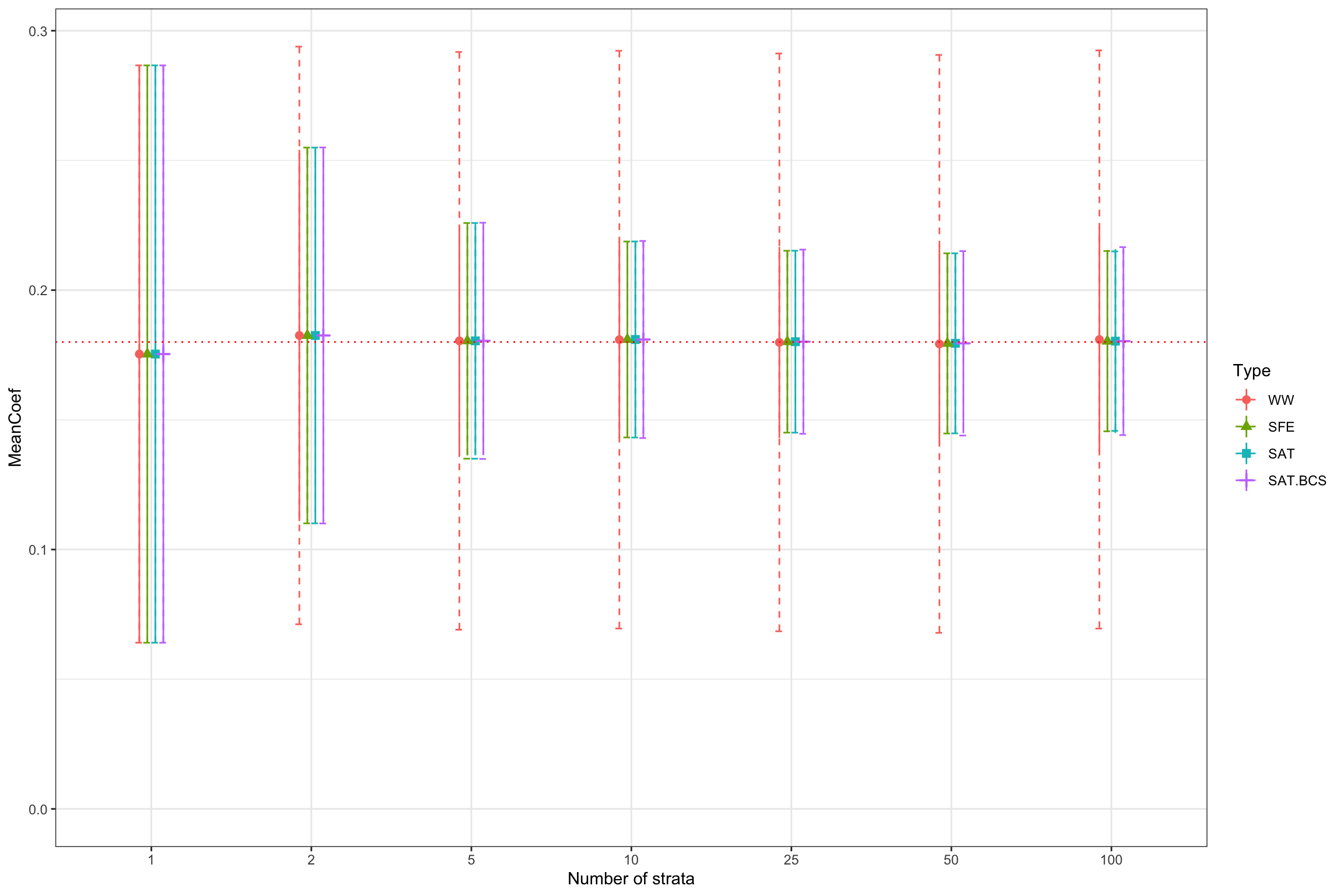
Figure 16.4: Distribution of estimators under various levels of stratification and estimated sampling noise (dashed lines)
As expected, the fully saturated model performs very well at estimating the actual level of sampling noise. Note that the default OLS estimator of sampling noise completely fails to reflect the precision gains due to stratification.
16.1.3.1.2 Estimating sampling noise of the strata fixed effects estimator
The strata fixed effects estimator is very similar to the fully saturated estimator, as Theorem 16.1 shows. They former differs only by having the proportion of treated and untreated in each strata appear in the formula for the weights. There are two key questions that one can then ask:
- What is the heteroskedasticity-consistent CLT-based approximation to the distribution of the strata fixed effects estimator?
- Does this distribution differ from the one of the fully saturated estimator and if yes how?
The following theorem answers the first question:
Theorem 16.5 (Asymptotic estimate of sampling noise of the strata fixed effects estimator) Under Assumptions 16.1, 16.2, 16.3, 16.4 and 16.5, the asymptotic distribution of the fully saturated estimator can be approximated as follows:
\[\begin{align*} \sqrt{N}\left(\hat{\beta}^{SFE}-\Delta^{Y}_{ATE}\right) & \distr \mathcal{N}\left(0,\sum_{s\in\mathcal{S}}\frac{(w^{SFE}_s)^2}{p_s}\left(\frac{\var{Y_i^1|R_i=1,\mathbf{s}(i)=s}}{\Pr(R_i=1|\mathbf{s}(i)=s)}+\frac{\var{Y_i^0|R_i=0,\mathbf{s}(i)=s}}{1-\Pr(R_i=1|\mathbf{s}(i)=s)}\right)\right). \end{align*}\]
Proof. See in Appendix A.7.5.
The following corollary answers the second question:
Corollary 16.1 (Equality of sampling noise for the strata fixed effects estimator and the fully saturated estimator) Under Assumptions 16.1, 16.2, 16.3, 16.4 and 16.5, and assuming that the proportion of treated units is equal to \(\pi\) in each strata, we have:
\[\begin{align*} \sqrt{N}\left(\hat{\beta}^{SFE}-\Delta^{Y}_{ATE}\right) & \distr \mathcal{N}\left(0,\sum_{s\in\mathcal{S}}p_s\left(\frac{\var{Y_i^1|R_i=1,\mathbf{s}(i)=s}}{\Pr(R_i=1)}+\frac{\var{Y_i^0|R_i=0,\mathbf{s}(i)=s}}{1-\Pr(R_i=1)}\right)\right). \end{align*}\]
Proof. If \(\bar{R}_s=\pi\), we have \(w^{SFE}_s=p^s\) and \(\Pr(R_i=1|\mathbf{s}(i)=s)=\Pr(R_i=1)\), under Assumption 16.5. Using Theorem 16.5 proves the result.
Remark. As a consequence, if the proportion of treated in each strata is roughly constant, both the strata fixed effect estimator and the fully saturated estimator will have similar sampling noise.
Remark. How to estimate the sampling noise of the strata fixed effect estimator?
Simply using the heteroskedasticity-robust estimator, for example the vcov="HC1" in feols, as we did in the numerical example above.
The estimates in Figure 16.4 suggest that this approach performs very well indeed.
16.1.3.1.3 Estimating sampling noise of the with/without estimator
What is the sampling noise of the WW estimator? How can we estimate it in practice? I leave the answers to these questions as an exercise. The OLS estimator is probably some weighted average of the \(\hat{\Delta}^Y_{WW_s}\) parameters, with weights that are going to drive the asymptotic distribution. Under plausible assumptions (constant strata poportions and constant proportion of treated), we probably get that its asymptotic distribution should be equal to that of the other two estimators. This is what Figure 16.4 suggests.
Remark. The default (even heteroskedasticity robust) standard error of the WW estimator estimated by OLS is NOT an adequate measure of sampling noise under stratification, since it does not account for the fact that stratification has reduced sampling noise by capturing part of the vaariation in potential outcomes. This appears clearly on Figure 16.4, where the estimated sampling noise of the WW estimator is always equal to the one without stratification. Ignoring stratification when estimating precision might leave a lot of precision on the table.
Remark. Figure 16.4 also shows another problem with the WW estimator: its precision starts decreasing when we increase the number of strata above 25. What is happening is that some strata start having no treated or no untreated units. The SAT and SFE estimators exclude these strata from the estimation (thereby biasing the final estimate) whereas the WW estimator do not exclude them and ends up using an unbalanced, noisier sample. Note that the standard errors that we used so far do not reflect that risk.
16.1.3.2 Estimating sampling noise under varying strata proportions
What happens when we relax Assumption 16.5, that is when we acknowledge that the proportion of observations in each strata might vary with \(N\)? The reason why this might happen is first because, in small samples, and with small strata, rounding errors might make the actual strata proportions far away from their theoretical values, even with stratified block randomization. Another reason is that we might use a stratification procedure that does not have the property of keeping strata proportions constant. A final reason is that we might be delimiting strata in a first step from a given sample, a thus strata are an estimated, whose true proportion in the population are unkwnown objects around which we can at best form a noisy estimator. This is for example the case when delimiting strata using \(k-\)means clustering as we did in our example.
Example 16.3 In order to illustrate the first source of failure of Assumption 16.5, let us plot the proportion of each strata in our samples, along with their theoretical values.
data.strata.prop <- data.strata %>%
                    mutate(
                      qs = Ns/N
                    ) %>%
                    group_by(strata_type,strata_value,strata_type_value) %>%
                    summarize(
                      qs = mean(qs)
                    ) %>%
                    mutate(
                      strata_type=factor(strata_type,levels=c(paste("strata",c(1,2,5,10,25,50,100),sep='_'))),
                      Nstrata = as.numeric(str_split_fixed(strata_type,'\\_',2)[,2]),
                      qsstar = 1/Nstrata
                    )
Let us plot the result:
ggplot(data.strata.prop %>% filter(strata_type!="strata_1",strata_type!="strata_2"),aes(x=qs))+
  geom_histogram(binwidth=0.01,color='black',fill='white')+
  geom_vline(aes(xintercept=qsstar),color='red',linetype='dashed')+
  xlim(0,0.35)+
  theme_bw() +
  facet_wrap(.~strata_type)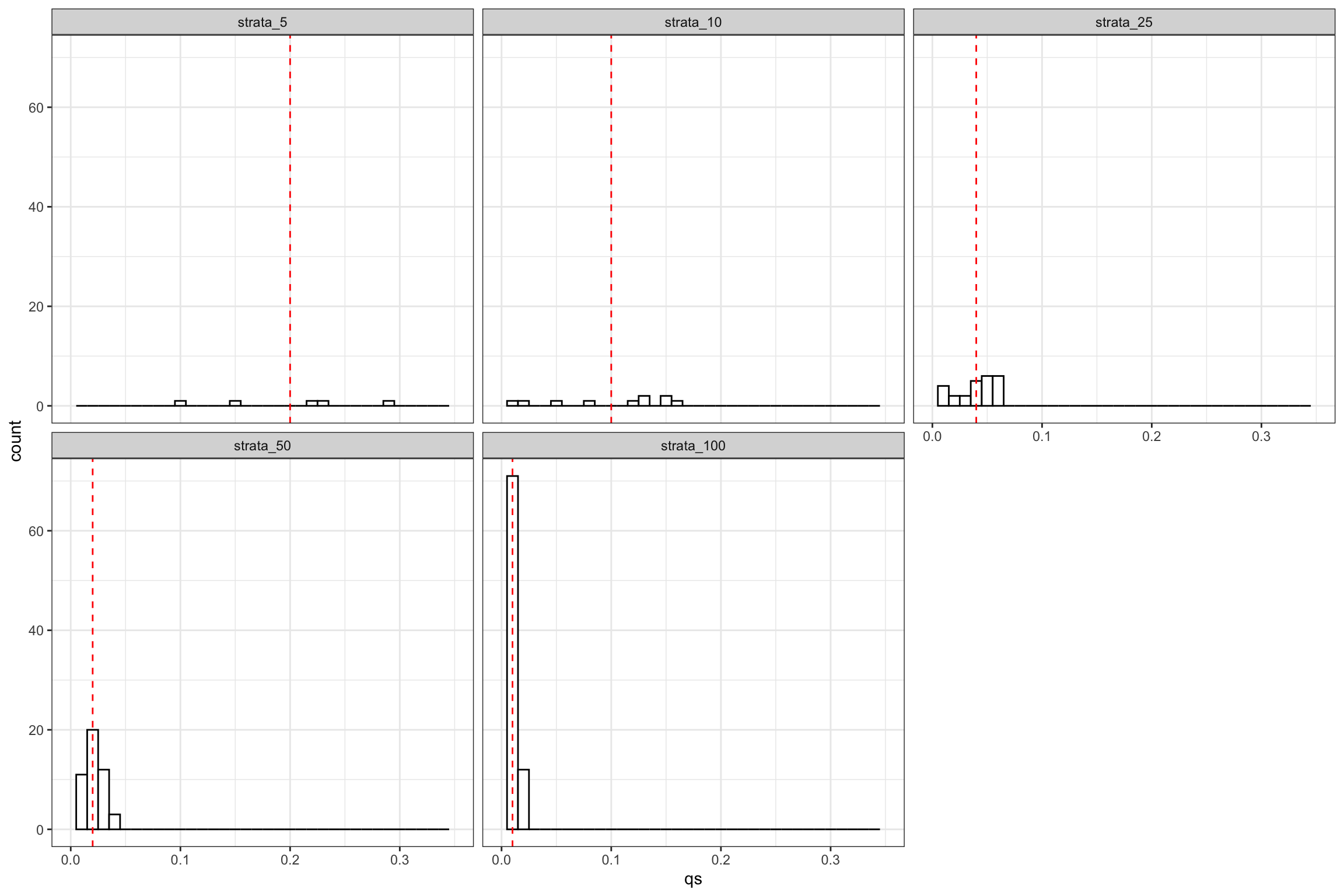
Figure 16.5: Strata proportions
As Figure 16.5 shows, there is substantial variation in a given sample around the theoretical strata proportion.
Remark. Note that it is not clear whether we would expect strata proportions to be constant at \(\frac{1}{S}\) with strata defined by \(k\)-means clustering. A more rigorous check would define strata as based on a finite set of threshold values on the support of \(\ln y_b\) and would derive the strata proportions in the population before checking the actual distribution of the proportion of these strata in each sample. We expect a substantial amount of variation. This is left as an exercise.
Remark. An even more difficult exercise would be to compute the strata proportions under \(k\)-means clustering. This is left as an exercise.
We are going to relax Assumption 16.5 by using instead the following assumption, suggested by Bugny, Canay and shaikh (2018):
Hypothesis 16.6 (Strong balance) We assume that
\[\begin{align*} \plims\frac{1}{\sqrt{N}}\sum_{i=1}^N(R_i-\pi)\uns{\mathbf{s}(i)=s}=0, \forall s\in\mathcal{S}. \end{align*}\]
Assumption of 16.6 imposes that the discrepancy between the proportion of treated in each strata and the target proportion \(\pi\) goes to zero faster than \(\sqrt{N}\). Assumption of 16.6 is satisfied with stratified block randomization, if the number of strata does not increase with \(N\). We can now state the following result:
Theorem 16.6 (Sampling noise under strong balance) Under Assumptions 16.1, 16.2, 16.3, 16.4 and 16.6, the asymptotic distribution of the fully saturated estimator of the strata fixed effects estimator can be approximated as follows:
\[\begin{align*} \sqrt{N}\left(\hat{\Delta}^Y_{SAT}-\Delta^{Y}_{ATE}\right) & \distr \mathcal{N}\left(0, \begin{array}{c} \sum_{s\in\mathcal{S}}p_s\left(\frac{\var{Y_i^1|R_i=1,\mathbf{s}(i)=s}}{\Pr(R_i=1|\mathbf{s}(i)=s)}+\frac{\var{Y_i^0|R_i=0,\mathbf{s}(i)=s}}{1-\Pr(R_i=1|\mathbf{s}(i)=s)}\right) \\ + \sum_{s\in\mathcal{S}}p_s\left(\esp{\esp{Y^1_i-Y^0_i|Z_i}-\esp{Y_i^1-Y^0_i}|\mathbf{s}(i)=s}\right)^2 \end{array} \right), \end{align*}\] where \(Z_i\) are the observed baseline covariates used to generate the strata.
Proof. See Bugni, Canay and Shaikh (2019) Theorems 3.1 and 3.2 applied to a single treatment (Section 5).
Theorem 16.6 shows that the asymptotic variance of the strata fixed effects and fully saturated estimators has two components: the first one is the one we are already familiar with under constant strata proportions, and the second one is a new component. This new component stems from the variance in treatment effects across strata. It can be estimated as follows:
\[\begin{align*} \hat{\mathbf{V}}_H & = \sum_{s=1}^S\frac{N_s}{N}(\hat{\beta}^{SAT}_s-\hat{\Delta}^Y_{WW})^2. \end{align*}\]
\(\hat{\mathbf{V}}_H\) estimates the variance in treatment effects across strata.
Example 16.4 Let’s see how the Bugni, Canay and Shaikh (2019) correction (adding \(\hat{\mathbf{V}}_H\) to our estimate of the asymptotic variance) changes our variance estimates. We have already implemented it in the Monte Carlo simulations. Figure 16.4 suggests that the correction does not make much of a difference in our example. It seems though that, with 100 strata, the standard errors without the correction are too tight and that the correction enables to recover correct estimates of sampling noise.
Remark. Bugni, Canay and Shaikh (2019) present simulations where their correction term makes an even greater difference.
Remark. Bugni, Canay and Shaikh (2019) also provide derivations for the case of multiple treatments.
16.1.3.3 Randomization inference for stratified experiments
Remark. Bugny, Canay and shaikh (2018) show in their Theorems 4.5 and 4.6 that randomization inference can recover adequate measures of precision under Assumption 16.6. Using randomization inference based on the t-stat build using the distribution in Theorem 16.6 is always consistent under Assumption 16.6. Using randomization inference based on the t-stat build using the distribution in Theorem 16.4 is consistent under Assumption 16.6 and with the additional requirement that \(\pi=0.5\).
16.2 Analysis of pairwise randomized controlled trials
With pairwise stratification, all strata are of size \(N_s=2\). There are several advantages to using paurwise stratification. With classical stratification, i.e. defining strata ex-ante, some strata might end up empty, populated by one unit of observation, etc. One solution to that issue is to use \(k\)-means clustering as we have done in the previous section, but that requires abandoning the constant strata proportion approach. But having strata that are of size superior to two suggests that we could increase precision by more by decreasing the size of the strata, trying to make units more and more similar. The limit of that process is to have strata of size two, with only one treated and one control observation in each. Of course, that reasoning probably puts under the carpet the classical bias/variance trade-off, and we will come back to that in the end of the section.
There are several challenges to implementing and analyzing a pairwise randomized controlled trial. The first of these challenges is the choice of the sample pairs. How do we choose the units that are closest to each other in the sample, so that some measure of the total discrepancy between pairs is minimized? This is actually not an easy problem to solve. In this section, I use recent results in operational research to help build the pairs, which tremendously decrease the time required to generate an adequate sample for randomization and make this approach much more feasible and usable than what it is now. The second challenge is the estimation of sampling noise. We indeed cannot use the formula in Theorem 16.4 and Theorem 16.5 because the variance of each potential outcome is not identified under within pairs (since we only have one observation of each potential outcome within the pair). A solution to that issue is to simply analyze the sample using pair fixed effects or pairwise differences.
16.2.1 Building a sample of pairs
A key difficulty in pairwise stratification is to build an adequate sample of pairs. It is so difficult that applied researchers in economics generally resort to a greedy approach: go through a large random sample of pairs and keep the one that is most satisfactory. One problem is that we do not know what satisfactory means: we need to choose a metric to measure of close all pairs are to each other. Here, I am going to use Euclidean or Mahalanobis distance, a measure of how different two observations are based on their observed covariates.
A second problem is that we do not know whether the resulting sample is actually the optimal one. It might not be. A third problem is that this approach is greedy: it takes time, so much time, and the time it requires increase exponentially with sample size (it is an NP-hard type of problem).
These last two issues can be solved in polynomial time using recent results in operations research.
The problem and how it has been solved are described on Joris van Rantwijk’s webpage.
The classical algorithm is Edmond’s Blossom algorithm.
Fortunately, Cole Beck recently imported the Blossom algorithm to R within the nbpMatching package.
In order to implement the pairing, we need a distance matrix between all possible pairs of units in the data.
The gendistance function of the nbpMatching package computes this matrix using the Mahalanobis distance.
Then, the Blossom algorithm is called using the nonbimatch command, after adequately transforming the matrix into a suitable input format using the distancematrix command.
Example 16.5 Let’s see how this all works in our example.
#N <- 6

# restrict to original dataset
data.strata.original <- data.strata %>%
                 filter(strata_type=="strata_1") %>% ungroup(.) %>% mutate(id=as.character(id))
# compute the distance matrix
#distance <- gendistance(data.strata.original %>% select(id,yB,y0),idcol=1)Remark. Unfortunately, I’ve ran into some technical issues with the implementation of the algorithm that I cannot solve right now.
Instead of using the Blossom algorithm to form the pair, I am going to order all observations by pre-treatment income, and form alternating pairs. With several treatment variables, one would have to build a score for all the variables (their weighted mean) and before ordering. Let’s go.
# random seed
set.seed(1234)
# restrict to original dataset
data.strata.original <- data.strata %>%
                 filter(strata_type=="strata_1") %>%
                 ungroup(.) %>%
                 select(-contains('strata'),-contains('rand'),-Ds,-y,-Ns,-pis) %>%
                 arrange(yB) %>%
                 mutate(
                   strata = rep(1:(N/2),2)[order(rep(1:(N/2),2))],
                   randU = runif(N)
                 )  %>%
                group_by(strata) %>%
                mutate(
                  randUMedStrata = stats::median(randU),
                  Ds = case_when(
                    randU<randUMedStrata ~ 1,
                    TRUE ~ 0
                  ),
                  y = y1*Ds+(1-Ds)*y0
                )
We now have a sample of 500 pairs, where each pair is composed of observations with similar \(y^B_i\).
16.2.2 Estimating treatment effects in pairwise randomized controlled trials
In order to estimate treatment effects in pairwise randomized controlled trials, we can use either the \(WW\) estimator, the strata fixed effects estimator or the fully saturated estimator. We also have that the last two estimators are actually identical (it follows from Theorems 16.1 and 16.3 with \(\bar{R}_s=\frac{1}{2}\), \(\forall s\)). There is actually another estimator that we might prefer to use, since it will give the correct estimator of sampling noise: the pairwise difference estimator.
The pairwise difference estimator works as follows. First we form the pairwise difference in outcomes: \(\Delta_s^Y=Y_{i\in\mathcal{I}(s)\land D_i=1}-Y_{j\in\mathcal{I}(s)\land D_j=0}\). Now, we simply regress the pairwise difference on a constant and estimate using OLS to obtain the estimated treatment effect:
\[\begin{align*} \Delta_s^Y & = \alpha^{PD} +\epsilon^{PD}_s. \end{align*}\]
We can prove the following theorem:
Theorem 16.7 (Unbiasedness and consistency of the pairwise difference estimator) Under Assumptions 3.1, 3.2 and 16.1, the pairwise difference estimator is an unbiased and consistent estimator of the Average Treatment Effect:
\[\begin{align*} \esp{\hat{\alpha}^{PD}} & = \Delta^Y_{ATE}\\ \plims\hat{\alpha}^{PD} & = \Delta^Y_{ATE}. \end{align*}\]
We also have that the pairwise difference estimator is numericalluy equivalent to the WW, SAT, and SFE estimators.
Proof. See in Appendix A.7.6.
Remark. It is also true that \(\hat\alpha^{WSD}=\frac{1}{\frac{N}{2}}\sum_{s=1}^S\Delta_s^Y\), the across-strata mean of the within strata differences. What is nice with the regression-based formulation is that it opens up the possibility of adding control variables:
\[\begin{align*} \Delta_s^Y & = \alpha^{WSD(X)} +\beta^{WSD(X)}\Delta_s^X +\gamma^{WSD(X)}(\bar{X}_s-\bar{X}) +\epsilon^{WSD(X)}_s, \end{align*}\]
where \(\bar{X}_s\) is the within strata mean of the covariates and \(\bar{X}\) is their overall sample mean.
Example 16.6 Let’s see how this works in our example. Let us first form the pairwise difference estimator and see how it compares to the other ones.
# PD
regPD <- data.strata.original %>%
        select(strata,Ds,y) %>%
        pivot_wider(names_from='Ds',values_from =  'y',names_prefix='y',names_sep='') %>%
        mutate(
          Deltay = y1-y0
        ) %>%
        lm(Deltay~1,data=.) %>%
        coef(.)

# WW
regWW <- data.strata.original %>%
        lm(y~Ds,data=.)%>%
        coef(.)

# strata fixed effects
regSFE <- data.strata.original %>%
          feols(y~Ds|strata,vcov="HC1",data=.)%>%
        coef(.)

# fully staturated model
# run a regression in each strata
regSAT <- data.strata.original %>%
          group_by(strata) %>%
          nest(.) %>%
          mutate(
            reg = map(data,~feols(y~Ds|1,vcov="HC1",data=.)),
            tidied = map(reg,tidy)
          ) %>%
          unnest(tidied) %>%
          filter(term == 'Ds') %>%
          rename(
            Coef = estimate,
            Se = std.error
          ) %>%
          mutate(
            qs = 2/N
          ) %>%
          select(strata,Coef,qs) %>%
          ungroup(.) %>%
          summarise(
           Coef = weighted.mean.nest(Coef~qs,data=.,na.rm=TRUE)
          )
As expected, we have the pairwise difference estimator which is equal to 0.165, the WW estimator which is equal to 0.165, the SFE estimator which is equal to 0.165 and the SAT estimator which is equal to 0.165.
16.2.3 Estimating sampling noise in pairwise randomized controlled trials
The key question now is how to estimate sampling noise for the pairwise difference estimator. One way to look at this issue would be to use results from Section 16.1, and especially Theorems 16.4 and 16.6. We thus have the classical result that sampling noise is the weighted average of the sum of variances of the potential outcomes in each strata plus, in the absence of constant strata proportions, the variance of treatment effects across strata. The problem we have is that, with only one treated and one untreated observation per strata, we cannot estimate the variance of the potential outcomes in each strata. We might be willing to use the default variance of the pairwise difference estimator, or the one of the strata fixed effects estimator, but without any knwoledge of whether they indeed work. So we seem stuck.
Fortunately, Bai, Romano and Shaikh (2021) have recently examined that issue in detail and have given us guidance. Bai, Romano and Shaikh (2021) require several assumptions to provide an answer to our problem. Before stating these assumptions, it is useful to reframe the pairing procedure as the \(\lfloor\frac{N}{2}\rfloor\) pairs such that \(\left\{\pi(2j-1),\pi(2j)\right\}\) for \(j\in\left\{1,\dots,\lfloor\frac{N}{2}\rfloor\right\}\), where \(\pi\) is a permutation of the \(N\) units in the sample based on \(\mathbf{X}\), the whole matrix of covariates in the sample. In a sense, we simply have ordered the observations in the sample so that consecutive observations are in the same pair. We are going to impose some restrictions on this permutation so that it is optimal in some sense:
Hypothesis 16.7 (Members of Each Pairs are Close) We assume that the members of the pairs generated by the pairing algorithm are close: \[\begin{align*} \plims\frac{1}{\lfloor\frac{N}{2}\rfloor}\sum_{j=1}^{\lfloor\frac{N}{2}\rfloor}\left|X_{\pi(2j)}-X_{\pi(2j-1)}\right|^r=0\text{, for }r=1\text{ and }r=2. \end{align*}\]
For estimating the variance, we will also use the fact that consecutive pairs are also close:
Hypothesis 16.8 (Consecutive Pairs are Close) We assume that the consecutive pairs generated by the pairing algorithm are close: \[\begin{align*} \plims\frac{1}{\lfloor\frac{N}{2}\rfloor}\sum_{j=1}^{\lfloor\frac{N}{4}\rfloor}\left|X_{\pi(4j-k)}-X_{\pi(4j-l)}\right|^2=0\text{, for any }k\in\left\{2,3\right\}\text{ and }l\in\left\{0,1\right\}. \end{align*}\]
We also need to formally assume that the allocation is random within pairs:
Hypothesis 16.9 (Randomized Allocation Within Pairs) We assume that treatment assignement is such that \((\mathbf{Y^1},\mathbf{Y^0})\Ind\mathbf{D}|\mathbf{X}\) and that, conditional on \(\mathbf{X}\), \(\left\{(D_{\pi(2j-1)},D_{\pi(2j))}\right\}_{j\in\left\{1,\dots,\lfloor\frac{N}{2}\rfloor\right\}}\) are i.i.d. and uniformly distributed over \(\left\{(0,1),(1,0)\right\}\).
Finally, we also need some to assume some restrictions on the potential outcomes:
Hypothesis 16.10 (Finite variance of potential outcomes) We assume that the distribution of potential outcomes in the population is such that:
- \(\esp{\var{Y_i^d|X_i}}>0\), for \(d\in\left\{0,1\right\}\)
- \(\esp{(Y^d_i)^2}<\infty\), for \(d\in\left\{0,1\right\}\)
- \(\esp{Y^d_i|X_i=x}\) and \(\esp{(Y^d_i)^2|X_i=x}\) are Lipschitz for \(d\in\left\{0,1\right\}\)
We can now state the following theorem:
Theorem 16.8 (Sampling noise under pairwise randomization) Under Assumptions 16.7, 16.9 and 16.10, the asymptotic distribution of pairwise difference estimator can be approximated as follows:
\[\begin{align*} \sqrt{N}\left(\hat{\alpha}^{PD}-\Delta^{Y}_{ATE}\right) & \distr \mathcal{N}\left(0, \begin{array}{c} \frac{\esp{\var{Y_i^1|X_i}}}{\frac{1}{2}}+\frac{\esp{\var{Y_i^0|X_i}}}{\frac{1}{2}}\\ + \esp{\left(\esp{Y^1_i-Y^0_i|X_i}-\esp{Y_i^1-Y^0_i}\right)^2} \end{array} \right). \end{align*}\]
Proof. See Bai, Romano and Shaikh (2021) Lemma S.1.4 in the Supplementary Appendix.
Remark. We recognize the first two elements of the variance formula in Theorem 16.8: they are the usual variances of the potential outcomes, net of the impavct of the covariates used to build the pairs. The last element takes into account of the fact that each time we take a new sample, we build new pairs, which generates variation in the average treatment effect that we estimate.
We now need to find estimators for the elements of the variance in Theorem 16.8. Bai, Romano and Shaikh (2021) propose several estimators, but the most closely linked to the theoretical result is the following:
\[\begin{align*} \hat\nu^2 & = \hat\varsigma^2+\hat\tau^2 \\ \hat\varsigma^2 & =\frac{1}{\lfloor\frac{N}{2}\rfloor}\sum_{l=1}^{\lfloor\frac{S}{2}\rfloor}\left(\Delta^Y_{\pi(2l)}-\Delta^Y_{\pi(2l-1)}\right)^2 \\ \hat\tau^2 & = \frac{1}{\lfloor\frac{N}{2}\rfloor}\sum_{s=1}^{S}\left(\Delta^Y_s-\hat\alpha^{PD}\right)^2 \end{align*}\]
\(\hat\varsigma^2\) is the average squared difference in pairwise treatment effects between consecutive pairs (note that the division is by \(\lfloor\frac{N}{2}\rfloor=S\) the total number of consecutive pairs, not by \(\lfloor\frac{N}{4}\rfloor=\lfloor\frac{S}{2}\rfloor\), the actual number of consecutive pairs of pairs. This component estimates the variance in treatment effects that is only due to unobserved covariates beyond \(X_i\), since consecutive pairs have very similar sets of observed covariates. \(\hat\tau^2\) measures the overall variance in treatment effects around the mean, again with the total sample size taken to normalize variances and not the number of pairs.
Example 16.7 Let’s see how this works in our example.
Let us first compute the second component estimating the variance due to the treatment effect varying with covariates \(\hat\tau^2\).
hattau2 <- data.strata.original %>%
                select(strata,Ds,y) %>%
                pivot_wider(names_from='Ds',values_from =  'y',names_prefix='y',names_sep='') %>%
                mutate(
                  Deltay = y1-y0
                ) %>%
                ungroup(.) %>%
                summarize(
                  hattau2 = var(Deltay)
                ) %>%
                pull(hattau2)
Let us now compute the value of \(\hat\varsigma^2\), the component of the variance due to variations in treatment effects triggered by unobserved covariates:
hatvarsigma2 <- data.strata.original %>%
                select(strata,Ds,y) %>%
                pivot_wider(names_from='Ds',values_from =  'y',names_prefix='y',names_sep='') %>%
                mutate(
                  Deltay = y1-y0
                ) %>%
                ungroup(.) %>%
                # pairs of close pairs
                mutate(
                   strata = rep(1:(N/4),2)[order(rep(1:(N/4),2))]
                ) %>%
                # choose the first one as being untreated and the second one treated, that does not change anything since difference is then squared
                mutate(
                   Ds = rep(c(0,1),N/4)
                ) %>%
                select(-y1,-y0) %>%
                # pivoting to take pairwise differences in treatment effects
                pivot_wider(names_from='Ds',values_from =  'Deltay',names_prefix='Deltay',names_sep='') %>%
                mutate(
                  DeltaDeltay = Deltay1-Deltay0
                ) %>%
                summarize(
                  RSS = sum(DeltaDeltay^2)
                ) %>%
                mutate(
                  hatvarsigma2=RSS/(N/2)
                ) %>%
                pull(hatvarsigma2)
Let us now sum the two components and take their square root to extract the estimated standard error for our pairwise difference estimator:
With 95% confidence, our estimate of the treatment effect using the pairwise design is therefore 0.17 \(\pm\) 0.03. 99% estimated sampling noise is therefore 0.09. This is very close to the level of sampling noise that remains when analyzing a classical stratified randomized controlled trial with 100 strata using the saturated model, as Figure 16.3 shows: 99% sampling noise is equal to 0.09 with 100 strata. Since pairwise randomization is the limit of taking an increasing number of strata, and sampling noise seems to level off at around 25 strata, this results makes a lot of sense. I leave running Monte Carlo simulations to check that the CLT approximation .
Remark. Estimating sampling noise using the formula in Theorem 16.8 is slightly more involved than reading the result of a regression. While I’m not aware that these estimators have been programmed in any software for now, Bai, Romano and Shaikh (2021)’s Theorem 3.2 shows that we can use a simpler estimator for sampling noise. Indeed, the default standard error of the simple pairwise difference OLS estimator (under homoskedasticity) provides a conservative estimate of the sampling noise of the pairwise difference estimator. It is conservative in the sense that it is larger than the true level of sampling noise, unless the covariates used for stratification do not matter for treatment effect heterogeneity (for example because the treatment effect is constant of your covariates are crappy at capturing variations in treatment effect heterogeneity). In that case, the default OLS standard error is a consistent estimator of the standard error of the pairwise difference estimator. Actually, the default standard error of the simple pairwise difference OLS estimator is equal to \(\sqrt{2\frac{\hat\tau^2}{N}}\).
Example 16.8 Let’s see how that works in our example.
# PD
regPDSummary <- data.strata.original %>%
        select(strata,Ds,y) %>%
        pivot_wider(names_from='Ds',values_from =  'y',names_prefix='y',names_sep='') %>%
        mutate(
          Deltay = y1-y0
        ) %>%
        lm(Deltay~1,data=.)
The fully OLS based pairwise difference estimate is equal to 0.17 \(\pm\) 0.03. 99% estimated sampling noise using the default OLS standard error in the pairwise regression is therefore 0.09. As we can see, in our application, using the default OLS standard errors or the more refined ones stemming from Theorem 16.8 deliver almost undistinguishable results (you have to go far into the digits to actually start finding a difference). That result starts making sense when you look at the formula for \(\hat\varsigma^2\): if treatment effects are not predicted well by covariates, it simply provides another estimator for half the variance of the treatment effect (all variation in treatment effects between similar pairs comes from variance in \(Y^1_i\) and \(Y_i^0\) that is not accounted for by covariates).
Remark. Abadie and Angrist (2008) show that \(\sqrt{2\frac{\hat\varsigma^2}{N}}\) provides an estimate of the standard error of the sample average treatment effect in pairwise randomized experiments. This estimate can be much smaller than the actual default OLS standard error, and even than the correct standard error based on Theorem 16.8.
Example 16.9 Let’s see how this works in our example.
We have \(\sqrt{\frac{2\hat\varsigma^2}{N}}=\) 0.02, which is almost identical to the default OLS-based estimate and to the correct estimate stemming from Theorem 16.8. We also have that \(\sqrt{\frac{2\hat\tau^2}{N}}=\) 0.02 which is exactly equal to the default OLS-based estimate, as expected.
Remark. Bai, Romano and Shaikh (2021) show in simulations and applications that you sometimes lose considerable precision by using the default standard errors of the OLS-based pairwise difference estimator. Things are not always as rosy as in our application. As a consequence, I would urge everyone to use the results of Theorem 16.8 instead of the default OLS standard errors. The default OLS ones will capture the gains in power due to reduction in the variance of outcomes, while the corrected ones from Theorem 16.8 will capture both these improvements and the ones due to a decrease in sampling noise stemming from variations in treatment effects over samples.
Remark. Randomization inference is also a possible way to estimate standard errors and obtain confidence intervals in pairwise randomized experiments. Theorem 3.5 in Bai, Romano and Shaikh (2021) shows that using the t-statistic based on Theorem 16.8 offers correct coverage. Inverting the test-statistic of repeated randomization inference under various assumptions for the value of the treatment effect as done in Section 9.1.3.5 is one way to obtain confidence intervals using randomization inference.
Remark. Randomization inference might yield imprecise confidence intervals because of the lumpyness of the choice of the grid for the hypothetized value of the treatment effect. In order to avoid that issue, the best approach is to solve numerically for the two bounds of the confidence interval using the fact that they are defined as solutions to nonlinear equations, as remarked by Ho and Imai (2006).
The nonlinear equation defining \(C_g^U\) and \(C_g^L\), the upper and lower bounds of the confidence interval, are defined as follows:
\[\begin{align*} f(C_g) & = \hat p(C_g)-0.05 =0, \end{align*}\]
where \(\hat p(C_g)=\Pr(\hat T_{RI}(C_g)\geq \hat T(C_g))\), \(\hat T_{RI}(C_g)\) is the distribution of the t-statistic under the null estimated by randomization inference, \(\hat T(C_g)\) is the true value of the test statistic under the null in the sample, and \(C_g^U\leq \hat \delta \leq C_g^L\). In order to solve \(f(C_g)=0\) for \(C_g^U\) and \(C_g^L\), we can use either the bisection method or Newton’s method adapted for when \(f'\) is unknown (i.e. the secant method) (see Judd (1998)).
For the Newton/secant method, we need to find two starting points, \(C_g^{L}(0)\) and \(C_g^{U}(0)\). I propose to use the extremities of the confidence intervals estimated using the OLS standard errors based on the Central Limit Theorem. We then compute \(C_g(k+1)=C_g(k)-f(C_g(k))\frac{C_g(k)-C_g(k-1)}{f(C_g(k))-f(C_g(k-1))}\), where \(C_g(-1)=\hat\alpha^{PD}\). We stop when \(|C_g(k)-C_g(k+1)|\leq\epsilon(1+|C_g(k+1)|)\). If \(|f(C_g(k+1))|\leq\psi\), we report \(C_g(k+1)\) as the result, otherwise, we report failure of convergence.
For the bisection method, we need to find four starting values \(C_g^{L,l}(0)\) and \(C_g^{L,u}(0)\) and \(C_g^{U,l}(0)\) and \(C_g^{U,u}(0)\) such that \(f(C_g^{L,l}(0))<0\) and \(f(C_g^{L,u}(0))>0\) and \(f(C_g^{U,l}(0))<0\) and \(f(C_g^{U,u}(0))>0\). I propose to start with \(C_g^{L,u}(0)=C_g^{U,l}(0)=\hat\alpha^{PD}\) and \(C_g^{L,l}(0)=\hat\alpha^{PD}-k\hat\sigma_{\hat\alpha^{PD}}\) and \(C_g^{U,lu}(0)=\hat\alpha^{PD}+k\hat\sigma_{\hat\alpha^{PD}}\), with \(k\) an appropriately big enough quantile of the standard normal, for example the 0.9995 quantile which is equal to 3.29 and \(\hat\sigma_{\hat\alpha^{PD}}\) an initial estimate of the standard error of the treatment effect, for example the default OLS one. Once we have the interval, we compute its mid-point, \(C_g^M(0)\) and we calculate \(f(C_g^M(0))\). We refine the bounds by replacing the bound with the same sign as the one of \(f(C_g^M)\) by \(C_g^M\). The other bound stays unchanged. We obtain \(C_g^{l}(1)\) and \(C_g^{u}(1)\). We keep updating until \(C_g^{u}(k)-C_g^{l}(k)\leq\epsilon(1+|C_g^{l}(k)|+|C_g^{u}(k)|)\) or \(f(C_g^{M}(k))\leq\psi\), with \(\epsilon\) and \(\psi\) pre-specified precision levels.
I leave the implementation of these methods as an exercise. In my own applications, I have found that the bisection method is more robust and always converges.
Remark. A key remaining question is whether we should use classical stratified designs or pairwise designs. Recently, Bai (2022) has shown that the pairwise design achieves maximum precision among the set of stratified designs where the probability of assignment is one half.
Remark. Another important question is how to optimally include covariates when analyzing stratified experiments. Cytrynbaum (2023a) shows how to make this choice optimally. In the pairwise randomized experiment, including covariates is optimal.
Remark. Another important question is how to optimally build our strata: which covariates to use, how to use pilot data to build the strata, for example. These key questions are examined by Cytrynbaum (2023b). Cytrynbaum (2023b) also provides estimators for the precision of treatment effects estimated after covariate adjusted selection of pairs and strata relfecting the full gain in precision due to stratification.