Chapter 4 Natural Experiments

Natural Experiments are situations due to the natural course of events that approximate the conditions of a randomized controlled trial. In the economists’ toolkit, we generally make a distinction between:

Instrumental variables (IV), that rely on finding a plausibly exogeneous source of variation in treatment intake.
Regression Discontinuity Designs (RDD), that exploit a discontinuity in the eligibility to the treatment.
Difference In Differences (DID), that make use of the differential exposure of some groups to the treatment of interest over time.

Remark. The term Natural Experiments seems to be mostly used by economists. It dates back to Haavelmo (1944)’s paper on the Probability Approach to Econometrics, where he makes a distinction between the experiments we’d like to make as social scientists and the experiments that Nature provides us with, that are in general a subset of the experiments we’d like to make. This raises the question of our ability to identify the relationships of interest from the variation that is present in the data, a traditional problem in classical econometrics that has echoes in treatment effect estimation, where we also try to identify treatment effect parameters. At the time of Haavelmo, and until the beginning of the 1990s, there was no real discussion of the plausibility of the identifying assumptions (or restrictions) required for identification of certain relations, outside of a discussion of their theoretical plausiblility. With the credibility revolution brought about by Angrist (1990)’s paper and summarized in Angrist and Krueger (2001)’s review paper, the notion of natural experiment made a come back, with the idea that we might be able to look for specific set of events produced by Nature that more credibly identify a relationship of interest, i.e. that closely approximate true experimental conditions.

Remark. Outside of economics, Natural Experiments have also flourished, but without the term, and were compiled in the early textbook on research methods by Campbell (1966). Both Difference In Differences and Regression Discontinuity Designs have been actually developed outside of economics, mostly in education research. Instrumental Variables have had a separate history in economics and in genetics, were it is called the method of path coefficients.

4.1 Instrumental Variables

Instrumental Variables rely on finding a plausibly exogeneous source of variation in treatment intake. In the simple case of a binary instrument, the identification and estimation parts are actually identical to Encouragements designs in RCTs, that we have already studied in Section 3.4. As a consequence, unless we make very strong assumptions, an IV design is going to recover a Local Average Treatment Effect. Our classical assumptions are going to show up again: Independence, Exclusion Restriction, Monotonicity.

Remark. Examples of Instrumental Variables are:

Distance to college or to school for studying the impact of college or school enrollement on education, earnings and other outcomes.
Random draft lottery number for investigating the impact of military experience on earnings and other outcomes.
Randomized encouragement to participate in order to study the impact of a program.

Remark. The crucial part of an IV design is to justify the credibility of the exclusion restriction and independence assumptions. It is in general very difficult to justify these assumptions, especially the exclusion restriction assumption. In the examples above, one could argue that schools or colleges might be built where they are necessary, i.e. close to destitute populations, or, on the contrary, that they are built far from difficult neighbourhoods. As soon as distance to school becomes correlated with other determinants of schooling, such as parental income and education, the independence assumption is violated.

Even if school placement is truly independent of potential education and earnings outcomes at first, parents, by choosing where to live, will sort themselves such as the parents that pay more attention to education end up located closer to school. As a consequence, the independence assumption might be violated again.

Even when the instrument is truly random, such as a draft lottery number, and thus the independence assumption seems fine, the instrument may directly affect the outcomes by other ways than the treatment of interest. For example, receiving a low draft lottery number makes one more likely to be drafted. In response, one might decide to increase their length of stay in college in order to use the waiver for the draft reserved for students. If receiving a low draft lottery number increases the number of years of education, and in turn subsequent earnings, then the exclusion restriction assumption is violated.

In this section, I’m going to denote $Z_i$ a binary instrument that can either take value $0$ or $1$. In general, we try to reserve the value $1$ for the instrument value that increases participation in the treatment of interest. In our examples, that would be when for example, the distance to college is low, the draft lottery number is low, or someone receives an encouragement to enter a program.

4.1.1 An example where Monotonicity does not hold

Since Monotonicity is going to play such a particular role, and since we have already explored this assumption a little in Chapter 3, I am going to use as an example a model where the Monotonicity assumption actually does not hold. It will, I hope, help us understand better the way Monotonicity works and how it interacts with the other assumptions. The key component of the model that makes Monotonicity necessary is the fact that treatment effects are heterogeneous and correlated with participation in the treatment. We’ll see later that Monotonicity is unnecessary when treatment effects are orthogonal to take up.

Example 4.1 Let’s see how we can generate a model without Monotonicity:

\[\begin{align*} y_i^1 & = y_i^0+\bar{\alpha}+\theta\mu_i+\eta_i \\ y_i^0 & = \mu_i+\delta+U_i^0 \\ U_i^0 & = \rho U_i^B+\epsilon_i \\ y_i^B & =\mu_i+U_i^B \\ U_i^B & \sim\mathcal{N}(0,\sigma^2_{U}) \\ D_i & = \uns{y_i^B+\kappa_i Z_i + V_i\leq\bar{y}} \\ \kappa_i & = \begin{cases} -\bar{\kappa} & \text{ if } \xi_i = 1 \\ \underline{\kappa} & \text{ if } \xi_i = 0 \end{cases} \\ \xi & \sim\mathcal{B}(p_{\xi}) \\ V_i & = \gamma(\mu_i-\bar{\mu}) + \omega_i \\ (\eta_i,\omega_i) & \sim\mathcal{N}(0,0,\sigma^2_{\eta},\sigma^2_{\omega},\rho_{\eta,\omega}) \\ Z_i & \sim\mathcal{B}(p_Z) \\ Z_i & \Ind (y_i^0,y_i^1,y_i^B,V_i) \\ \xi_i & \Ind (y_i^0,y_i^1,y_i^B,V_i,Z_i) \end{align*}\]

The key component of the model that generates a failure of Monotonicity is the coefficient $\kappa_i$, that determines how individuals’ participation into the program reacts to the instrument $Z_i$. $\kappa_i$ is a coefficient whose value varies accross the population. In my simplified model, $\kappa_i$ can take only two values, $-\bar{\kappa}$ or $\underline{\kappa}$. When $-\bar{\kappa}$ and $\underline{\kappa}$ have opposite signs (let’s say $-\bar{\kappa}<0$ and $\underline{\kappa}>0$), then individuals with $\kappa_i=-\bar{\kappa}$ are going to be more likely to enter the program when they receive an encouragement (when $Z_i=1$) while individuals with $\kappa_i=\underline{\kappa}$ will be less likely to enter the program when $Z_i=1$. When $-\bar{\kappa}$ and $\underline{\kappa}$ have different signs, we have four types of reactions when the instrumental variable moves from $Z_i=0$ to $Z_i=1$, holding everything else constant. These four types of reactions define four types of individuals:

Always takers ($T_i=a$): individuals that participate in the program both when $Z_i=0$ and $Z_i=1$.
Never takers ($T_i=n$): individuals that do not participate in the program both when $Z_i=0$ and $Z_i=1$.
Compliers ($T_i=c$): individuals that do not participate in the program when $Z_i=0$ but that participate in the program when $Z_i=1$ .
Defiers ($T_i=d$): individuals that participate in the program when $Z_i=0$ but that do not participate in the program when $Z_i=1$ .

In our model, these four types are a function of $y_i^B+V_i$ and $\kappa_i$. In order to see this let’s define, as in Section 3.4, $D^z_i$ the participation decision of individual $i$ when the instrument is exogenously set to $Z_i=z$, with $z\in\left\{0,1\right\}$. When $\kappa_i=-\bar{\kappa}<0$, we have three types of reactions to the instrument. It turns out that each of type can be defined by where $y_i^B+V_i$ lies with respect to a series of thresholds:

Always takers ($T_i=a$) are such that $D^1_i=\uns{y_i^B-\bar{\kappa} + V_i\leq\bar{y}}=1$ and $D^0_i=\uns{y_i^B + V_i\leq\bar{y}}=1$, so that they actually are such that: $y_i^B+V_i\leq\bar{y}$. This is because $y_i^B+V_i\leq\bar{y} \Rightarrow y_i^B+V_i\leq\bar{y}+\bar{\kappa}$, when $\bar{\kappa}>0$.
Never takers ($T_i=n$) are such that $D^1_i=\uns{y_i^B-\bar{\kappa} + V_i\leq\bar{y}}=0$ and $D^0_i=\uns{y_i^B + V_i\leq\bar{y}}=0$, so that they actually are such that: $y_i^B+V_i>\bar{y}+\bar{\kappa}$. This is because $y_i^B+V_i>\bar{y}+\bar{\kappa} \Rightarrow y_i^B+V_i>\bar{y}$, when $\bar{\kappa}>0$.
Compliers ($T_i=c$) are such that $D^1_i=\uns{y_i^B-\bar{\kappa} + V_i\leq\bar{y}}=1$ and $D^0_i=\uns{y_i^B + V_i\leq\bar{y}}=0$, so that they actually are such that: $\bar{y}<y_i^B+V_i\leq\bar{y}+\bar{\kappa}$.

When $\kappa_i=\underline{\kappa}>0$, we have three types defined by where $V_i$ lies with respect to a series of thresholds:

Always takers ($T_i=a$) are such that $D^1_i=\uns{y_i^B+\underline{\kappa} + V_i\leq\bar{y}}=1$ and $D^0_i=\uns{y_i^B + V_i\leq\bar{y}}=1$, so that they actually are such that: $y_i^B+V_i\leq\bar{y}-\underline{\kappa}$. This is because $y_i^B+V_i\leq\bar{y}-\underline{\kappa} \Rightarrow y_i^B+V_i\leq\bar{y}$, when $\underline{\kappa}>0$.
Never takers ($T_i=n$) are such that $D^1_i=\uns{y_i^B-\bar{\kappa} + V_i\leq\bar{y}}=0$ and $D^0_i=\uns{y_i^B + V_i\leq\bar{y}}=0$, so that they actually are such that: $y_i^B+V_i>\bar{y}$. This is because $y_i^B+V_i>\bar{y} \Rightarrow y_i^B+V_i\leq\bar{y}-\underline{\kappa}$, when $\underline{\kappa}>0$.
Defiers ($T_i=d$) are such that $D^1_i=\uns{y_i^B+\underline{\kappa} + V_i\leq\bar{y}}=0$ and $D^0_i=\uns{y_i^B + V_i\leq\bar{y}}=1$, so that they actually are such that: $\bar{y}-\underline{\kappa}<V_i+y_i^B\leq\bar{y}$.

Let’s visualize how this works in a plot. Before that, let’s generate some data according to this process. For that, let’s choose values for the new parameters.

param <- c(8,.5,.28,1500,0.9,0.01,0.05,0.05,0.05,0.1,0.1,7.98,0.5,1,0.5,0.9,0.28,0)
names(param) <- c("barmu","sigma2mu","sigma2U","barY","rho","theta","sigma2epsilon","sigma2eta","delta","baralpha","gamma","baryB","pZ","barkappa","underbarkappa","pxi","sigma2omega","rhoetaomega")

set.seed(1234)
N <-1000
cov.eta.omega <- matrix(c(param["sigma2eta"],param["rhoetaomega"]*sqrt(param["sigma2eta"]*param["sigma2omega"]),param["rhoetaomega"]*sqrt(param["sigma2eta"]*param["sigma2omega"]),param["sigma2omega"]),ncol=2,nrow=2)
eta.omega <- as.data.frame(mvrnorm(N,c(0,0),cov.eta.omega))
colnames(eta.omega) <- c('eta','omega')
mu <- rnorm(N,param["barmu"],sqrt(param["sigma2mu"]))
UB <- rnorm(N,0,sqrt(param["sigma2U"]))
yB <- mu + UB 
YB <- exp(yB)
Ds <- rep(0,N)
Z <- rbinom(N,1,param["pZ"])
xi <- rbinom(N,1,param["pxi"]) 
kappa <- ifelse(xi==1,-param["barkappa"],param["underbarkappa"])
V <- param["gamma"]*(mu-param["barmu"])+eta.omega$omega
Ds[yB+kappa*Z+V<=log(param["barY"])] <- 1 
epsilon <- rnorm(N,0,sqrt(param["sigma2epsilon"]))
U0 <- param["rho"]*UB + epsilon
y0 <- mu +  U0 + param["delta"]
alpha <- param["baralpha"]+  param["theta"]*mu + eta.omega$eta
y1 <- y0+alpha
Y0 <- exp(y0)
Y1 <- exp(y1)
y <- y1*Ds+y0*(1-Ds)
Y <- Y1*Ds+Y0*(1-Ds)

We can now define the types variable $T_i$:

D1 <- ifelse(yB+kappa+V<=log(param["barY"]),1,0)
D0 <- ifelse(yB+V<=log(param["barY"]),1,0)
AT <- ifelse(D1==1 & D0==1,1,0)
NT <- ifelse(D1==0 & D0==0,1,0)
C <- ifelse(D1==1 & D0==0,1,0)
D <- ifelse(D1==0 & D0==1,1,0)
Type <- ifelse(AT==1,'a',
            ifelse(NT==1,'n',
                   ifelse(C==1,'c',
                          ifelse(D==1,'d',""))))

data.non.mono <- data.frame(cbind(Type,C,NT,AT,D1,D0,Y,y,Y1,Y0,y0,y1,yB,alpha,U0,eta.omega$eta,epsilon,Ds,kappa,xi,Z,mu,UB))

#ggplot(data.non.mono, aes(x=V, y=yB),color(as.factor(Type))) +
#    geom_point(shape=1)+
#    facet_grid(.~ as.factor(kappa))

plot(yB[AT==1 & kappa==-param["barkappa"]]+V[AT==1 & kappa==-param["barkappa"]],y[AT==1 & kappa==-param["barkappa"]],pch=1,xlim=c(5,11),ylim=c(5,11),xlab='yB+V',ylab="Outcomes")
points(yB[NT==1 & kappa==-param["barkappa"]]+V[NT==1 & kappa==-param["barkappa"]],y[NT==1 & kappa==-param["barkappa"]],pch=1,col='blue')
points(yB[C==1 & kappa==-param["barkappa"]]+V[C==1 & kappa==-param["barkappa"]],y[C==1 & kappa==-param["barkappa"]],pch=1,col='red')
points(yB[D==1 & kappa==-param["barkappa"]]+V[D==1 & kappa==-param["barkappa"]],y[D==1 & kappa==-param["barkappa"]],pch=1,col='green')
abline(v=log(param["barY"]),col='red')
abline(v=log(param["barY"])+param['barkappa'],col='red')
#abline(v=log(param["barY"])-param['underbarkappa'],col='red')
text(x=c(log(param["barY"]),log(param["barY"])+param['barkappa']),y=c(5,5),labels=c(expression(bar('y')),expression(bar('y')+bar(kappa))),pos=c(2,4),col=c('red','red'),lty=c('solid','solid'))
legend(5,10.5,c('AT','NT','C','D'),pch=c(1,1,1,1),col=c('black','blue','red','green'),ncol=1)
title(expression(kappa=bar(kappa)))

plot(yB[AT==1 & kappa==param["underbarkappa"]]+V[AT==1 & kappa==param["underbarkappa"]],y[AT==1 & kappa==param["underbarkappa"]],pch=1,xlim=c(5,11),ylim=c(5,11),xlab='yB+V',ylab="Outcomes")
points(yB[NT==1 & kappa==param["underbarkappa"]]+V[NT==1 & kappa==param["underbarkappa"]],y[NT==1 & kappa==param["underbarkappa"]],pch=1,col='blue')
points(yB[C==1 & kappa==param["underbarkappa"]]+V[C==1 & kappa==param["underbarkappa"]],y[C==1 & kappa==param["underbarkappa"]],pch=1,col='red')
points(yB[D==1 & kappa==param["underbarkappa"]]+V[D==1 & kappa==param["underbarkappa"]],y[D==1 & kappa==param["underbarkappa"]],pch=1,col='green')
abline(v=log(param["barY"]),col='red')
#abline(v=log(param["barY"])-param['barkappa'],col='red')
abline(v=log(param["barY"])-param['underbarkappa'],col='red')
text(x=c(log(param["barY"]),log(param["barY"])-param['underbarkappa']),y=c(5,5),labels=c(expression(bar('y')),expression(bar('y')-underbar(kappa))),pos=c(2,2),col=c('red','red'),lty=c('solid','solid'))
legend(5,10.5,c('AT','NT','C','D'),pch=c(1,1,1,1),col=c('black','blue','red','green'),ncol=1)
title(expression(kappa=underbar(kappa)))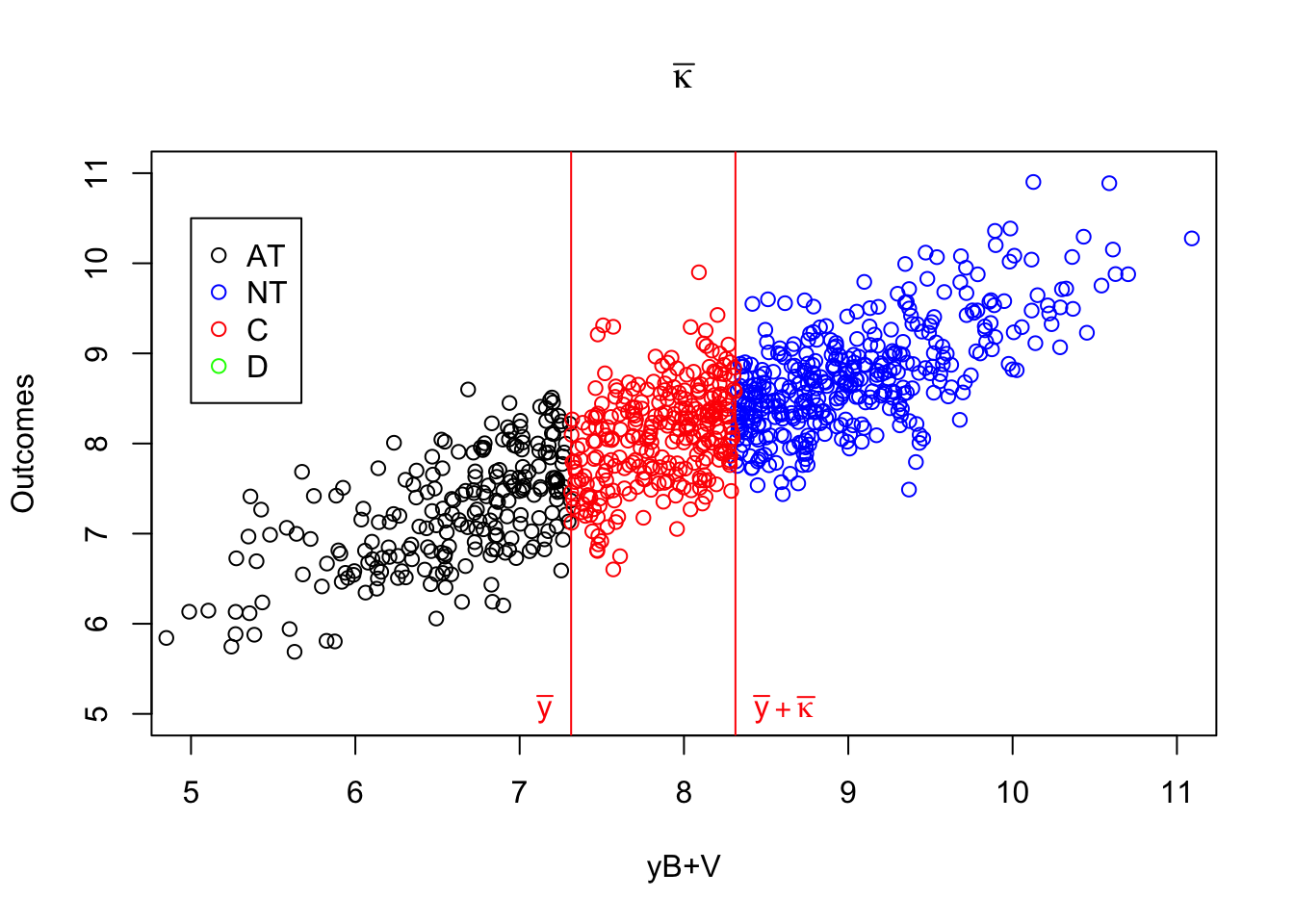

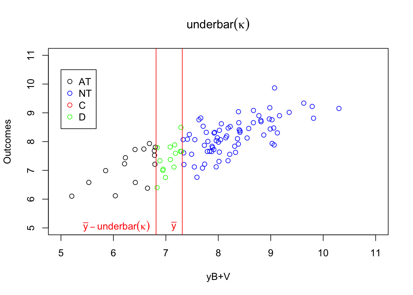
Figure 4.1: Types

As Figure 4.1 shows how the different types interact with $\kappa_i$. When $\kappa_i=-\bar{\kappa}$, individuals with $y_i^B+V_i$ below $\bar{y}$ always take the program. Even when $Z_i=1$ and $\bar{\kappa}$ is subtracted from their index, it is still low enough so that they get to participate. When $y_i^B+V_i$ is in between $\bar{y}$ and $\bar{y}+\bar{\kappa}$, the individuals are such that their index without subtracting $\bar{\kappa}$ is above $\bar{y}$, but it is below $\bar{y}$ when $\bar{\kappa}$ is subtracted from it. These individuals participate when $Z_i=1$ and do not participate when $Z_i=0$: they are compliers. Individuals such that $y_i^B+V_i$ is above $\bar{y}+\bar{\kappa}$ will have an index above $\bar{y}$ whether we substract $\bar{\kappa}$ from it or not. They are never takers.

When $\kappa_i=\underline{\kappa}$, individuals with $y_i^B+V_i$ below $\bar{y}-\underline{\kappa}$ always take the program. Even when $Z_i=0$ and $\underline{\kappa}$ is not subtracted from their index, it is still low enough so that they get to participate. When $y_i^B+V_i$ is in between $\bar{y}-\underline{\kappa}$ and $\bar{y}$, the individuals are such that their index without adding $\underline{\kappa}$ is below $\bar{y}$, but it is above $\bar{y}$ when $\underline{\kappa}$ is added to it. These individuals participate when $Z_i=0$ and do not participate when $Z_i=1$: they are defiers. Individuals such that $y_i^B+V_i$ is above $\bar{y}$ will have an index above $\bar{y}$ whether we add $\underline{\kappa}$ from it or not. They are never takers.

4.1.2 Identification

We need several assumptions for identification in an Instrumental Variable framework. We are going to explore two sets of assumption that secure the identification of two different parameters:

The Average Treatment Effect on the Treated ($TT$): identification will happen through the assumption of independence of treatment effects from potential treatment choice
The Local Average Treatment Effect ($LATE$)

Hypothesis 4.1 (First Stage Full Rank) We assume that the instrument $Z_i$ has a direct effect on treatment participation:

\[\begin{align*} \Pr(D_i=1|Z_i=1)\neq\Pr(D_i=1|Z_i=0). \end{align*}\]

Example 4.2 Let’s see how this assumption works in our example. Let’s first compute the average values of $Y_i$ and $D_i$ as a function of $Z_i$, for later use.

means.IV <- c(mean(Ds[Z==0]),mean(Ds[Z==1]),mean(y0[Z==0]),mean(y0[Z==1]),mean(y[Z==0]),mean(y[Z==1]),0,1)
means.IV <- matrix(means.IV,nrow=2,ncol=4,byrow=FALSE,dimnames=list(c('Z=0','Z=1'),c('D','y0','y','Z')))
means.IV <- as.data.frame(means.IV)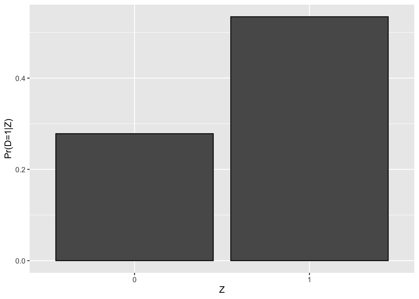

Figure 4.2: Proportion of participants as a function of $Z_i$

Figure 4.2 shows that the proportion of treated when $Z_i=1$ in our sample is equal to 0.53 while the proportion of treated when $Z_i=0$ is equal to 0.28, in accordance with Assumption 4.1. In the population, the proportion of treated when $Z_i=1$ depends on the value of $\kappa_i$. Let’s derive its value:

\[\begin{align*} \Pr(D_i=1|Z_i=1) & = \Pr(y_i^B+\kappa_i Z_i + V_i\leq\bar{y}|Z_i=1) \\ & = \Pr(y_i^B+\kappa_i + V_i\leq\bar{y}) \\ & = \Pr(y_i^B+ V_i\leq\bar{y}+\bar{\kappa}|\xi_i=1)\Pr(\xi_i=1) + \Pr(y_i^B+V_i\leq\bar{y}-\underline{\kappa}|\xi_i=0)\Pr(\xi_i=0) \\ & = \Pr(y_i^B+ V_i\leq\bar{y}+\bar{\kappa})p_{\xi} + \Pr(y_i^B+ V_i\leq\bar{y}-\underline{\kappa})(1-p_{\xi}) \\ & = p_{\xi}\Phi\left(\frac{\bar{y}+\bar{\kappa}-\bar{\mu}}{\sqrt{(1+\gamma^2)\sigma^2_{\mu}+\sigma^2_{U}+\sigma^2_{\omega}}}\right) + (1-p_{\xi})\Phi\left(\frac{\bar{y}-\underline{\kappa}-\bar{\mu}}{\sqrt{(1+\gamma^2)\sigma^2_{\mu}+\sigma^2_{U}+\sigma^2_{\omega}}}\right) \end{align*}\]

where the second equality follows from $Z_i$ being independent of $(y_i^0,y_i^1,y_i^B,V_i)$, the third equality follows from $\xi_i$ being independent from $(y_i^0,y_i^1,y_i^B,V_i,Z_i)$ and the last equality follows from the formula for the cumulative of a normal distribution. The formula for $\Pr(D_i=1|Z_i=0)$ is the same except for $\bar{\kappa}$ and $\underline{\kappa}$ that are set to zero.

Let’s write two functions to compute these probabilities:

prob.D.Z.1 <- function(param){
  part.1 <- param['pxi']*pnorm((log(param["barY"])+param['barkappa']-param['barmu'])/sqrt((1+param['gamma']^2)*param['sigma2mu']+param["sigma2U"]+param['sigma2omega']))
  part.2 <- (1-param['pxi'])*pnorm((log(param["barY"])-param['underbarkappa']-param['barmu'])/sqrt((1+param['gamma']^2)*param['sigma2mu']+param["sigma2U"]+param['sigma2omega']))
  return(part.1+part.2)
}
prob.D.Z.0 <- function(param){
  part.1 <- param['pxi']*pnorm((log(param["barY"])-param['barmu'])/sqrt((1+param['gamma']^2)*param['sigma2mu']+param["sigma2U"]+param['sigma2omega']))
  part.2 <- (1-param['pxi'])*pnorm((log(param["barY"])-param['barmu'])/sqrt((1+param['gamma']^2)*param['sigma2mu']+param["sigma2U"]+param['sigma2omega']))
  return(part.1+part.2)
}

With these functions, we know that, in the population, $\Pr(D_i=1|Z_i=1)=$ 0.57 and $\Pr(D_i=1|Z_i=0)=$ 0.25, which is not far from what we have found in our sample.

Our next set of assumptions imposes that the instrument has no direct effect on the outcome and that it is not correlated with all the potential outcomes. Let’s start with the exclusion restriction:

Hypothesis 4.2 (Exclusion Restriction) We assume that there is no direct effect of $Z_i$ on outcomes:

\[\begin{align*} \forall d,z \in \left\{0,1\right\}\text{, } Y_i^{d,z} = Y_i^d. \end{align*}\]

Example 4.3 In our example, this assumption is automatically satisfied.

Indeed, $y_i^{d,z}=y_i^0 + d(y_i^1-y_i^0)$ which is parameterized as $y_i^{d,z}=\mu_i+\delta+U_i^0+d(\bar{\alpha}+\theta\mu_i+\eta_i)$. Since $y_i^{d,z}$ does not depend on $z$, we have $y_i^{d,z} = y_i^d$, $\forall d,z \in \left\{0,1\right\}$. The assumption would not be satisfied if $Z_i$ entered the equations for $y_i^0$ or $y_i^1$. For example, if $Z_i$ is the Vietnam draft lottery number (high or low) used by Angrist to study the impact of army experience on earnings, the exclusion restriction would not work if $Z_i$ was directly influencing outcomes, independent of miitary experience, by example by generating a higher education level. In that case, we could have $E_i=\alpha+\beta Z_i + v_i$, where $E_i$ is education, and, for example, $y_i^0=\mu_i+\delta+\lambda E_i+U_i^0$. We then have $y_i^{d,z}=\mu_i+\delta +\lambda(\alpha+\beta z + v_i) +U_i^0+d(\bar{\alpha}+\theta\mu_i+\eta_i)$ which depends on $z$ and thus the exclusion restriction does not hold any more.

Let us now state the independence assumption:

Hypothesis 4.3 (Independence) We assume that $Z_i$ is independent from the other determinants of $Y_i$ and $D_i$:

\[\begin{align*} (Y_i^1,Y_i^0,D_i^1,D_i^0)\Ind Z_i. \end{align*}\]

Remark. Why do we say that independence from the potential outcomes is the same as independence from the other determinants of $Y_i$ and $D_i$? Because the only sources of variation that remain in $Y_i^d$ and $D_i^z$ are the other sources of variations (that is not the treatment $D_i=d$ nor the instrument variable $Z_i=z$).

Example 4.4 In our example, this assumption is also satisfied.

If we assumed that unobserved determinants of earnings contained in $U^0_i$ are correlated with the instrument value, then we would have a problem. For example, if children that leave close to college have also rich parents, or parents that spend a lot of time with them, or parents with large networks, there probably is a correlation between distance to college and earnings in the absence of the program. For the draft lottery example, you might have that people with a high draft lottery number who have well-connected parents obtain discharges on special medical grounds. Is that a violation of the independence assumption? Actually no. Indeed, these individuals are simply going to become never takers (they avoid the draft whatever their lottery number). But $Z_i$ is still independent from the level of connections of the parents. For the independence assumption to fail in the draft lottery number example, you would need that children of well-connected parents obtain lower lottery numbers because the lottery is rigged. In that case, since well-connected individuals would have had higher earnings even absent the lottery, there is a negative correlation between $y_i^0$ and having a high draft lottery number ($Z_i$).

The last assumption we need in order to identify the Local Average Treatment Effect is that of Monotonicity. We already know this assumption:

Hypothesis 4.4 (Monotonicity) We assume that the instrument moves everyone in the population in the same direction:

\[\begin{align*} \forall i\text{, either } D^1_i\geq D_i^0 \text{ or } D^1_i\leq D_i^0. \end{align*}\]

Without loss of generality, we generally assume that $\forall i$, $D^1_i\geq D_i^0$. As a consequence, there are no defiers.

Example 4.5 In our example, this assumption is not satisfied.

There are defiers, as Figure 4.1 shows, when $\xi_i = 0$ and thus $\kappa_i=\underline{\kappa}$. Indeed, in that case, for the individuals who are such that $\bar{y}-\underline{\kappa}<y_i^B+V_i\leq\bar{y}$, we have $D^1_i=\uns{y_i^B+\underline{\kappa} + V_i\leq\bar{y}}=0$ and $D^0_i=\uns{y_i^B + V_i\leq\bar{y}}=1$. This would happen for example if some people would go to college less if their house is located closer to the college, maybe for example because they have a preference not to stay at their parents’ house.

Remark. Why are defiers a problem for the instrumental variable strategy? Because the Intention to Treat Effect that measures the difference in expected outcomes at the two levels of the instrument is going to be characterized by two-way flows in and out of the program, as we have already seen with Theorem 3.10. This means that some treatment effects will have negative weights in the ITE formula. In that case, you might have a negative Intention to Treat Effect despite the treatment having positive effects for everyone, or you might under estimate the true effect of the treatment. This matters only when the treatment effects are heterogeneous.

Example 4.6 Let us detail how non-monotonicity and the existence defiers act on the ITE in our example, since we now have defiers. The first very important thing to understand is that all the problems we have happend because treatment effects are heterogeneous AND they are correlated with the type of individuals: defiers and compliers do not have the same distribution of treatment effects and, case in point, they do not have the same average treatment effects. The average effects of the treatment on compliers and defiers are not the same. Let us first look at the distribution of treatment effects among compliers and defiers in the sample and in the population.

In order to derive the distribution of $\alpha_i$ conditional on Type in the population, we need to derive the joint distribution of $\alpha_i$ and $y_i^B+V_i$ and use the trmtvnorm package to recover its density when it is truncated. This distribution is normal and fully characterized by its mean and covariance matrix.

\[\begin{align*} (\alpha_i,y_i^B+V_i) & \sim \mathcal{N}\left(\bar{\alpha}+\theta\bar{\mu},\bar{\mu}, \left(\begin{array}{cc} \theta^2\sigma^2_{\mu}+\sigma^2_{\eta} & (\theta+\gamma)\sigma^2_{\mu}+\rho_{\eta,\omega}\sigma^2_{\eta}\sigma^2_{\omega}\\ (\theta+\gamma)\sigma^2_{\mu}+\rho_{\eta,\omega}\sigma^2_{\eta}\sigma^2_{\omega} & (1+\gamma^2)\sigma^2_{\mu}+\sigma^2_U+\sigma^2_{\omega}\\ \end{array} \right) \right) \end{align*}\]

Let us write a function to generate them.

mean.alpha.yBV <- c(param['baralpha']+param['theta']*param['barmu'],param['barmu'])
cov.alpha.yBV <- matrix(c((param['theta']^2)*param['sigma2mu']+param['sigma2eta'],
                          (param['theta']+param['gamma'])*param['sigma2mu']+param['rhoetaomega']*param['sigma2eta']*param['sigma2omega'],
                            (param['theta']+param['gamma'])*param['sigma2mu']+param['rhoetaomega']*param['sigma2eta']*param['sigma2omega'],
                            (1+param['gamma']^2)*param['sigma2mu']+param['sigma2U']+param['sigma2omega']),2,2,byrow=TRUE)
# density of alpha for compliers
lower.cut.comp <- c(-Inf,log(param['barY']))
upper.cut.comp <- c(Inf,log(param['barY'])+param['barkappa'])
d.alpha.compliers <- function(x){
  return(dtmvnorm.marginal(xn=x,n=1,mean=mean.alpha.yBV,sigma=cov.alpha.yBV,lower=lower.cut.comp,upper=upper.cut.comp))
}
# density of alpha for defiers
lower.cut.def <- c(-Inf,log(param['barY']-param['underbarkappa']))
upper.cut.def <- c(Inf,log(param['barY']))
d.alpha.defiers <- function(x){
  return(dtmvnorm.marginal(xn=x,n=1,mean=mean.alpha.yBV,sigma=cov.alpha.yBV,lower=lower.cut.def,upper=upper.cut.def))
}

Let us now plot the empirical and theoretical distributions of the treatment effects for compliers and defiers.

# building the data frame
alpha.types <- as.data.frame(cbind(alpha,C,D,AT,NT)) %>%
                mutate(
                  Type = ifelse(AT==1,"Always Takers",
                                ifelse(NT==1,"Never Takers",
                                       ifelse(C==1,"Compliers","Defiers")))
                ) %>%
                mutate(Type = as.factor(Type))

ggplot(filter(alpha.types,Type=="Compliers" | Type=="Defiers"), aes(x=alpha, colour=Type)) + 
  geom_density(linetype="dashed") +
  geom_function(fun = d.alpha.compliers, colour = "red") +
  geom_function(fun = d.alpha.defiers, colour = "blue") +
  ylab('density') +
  theme_bw()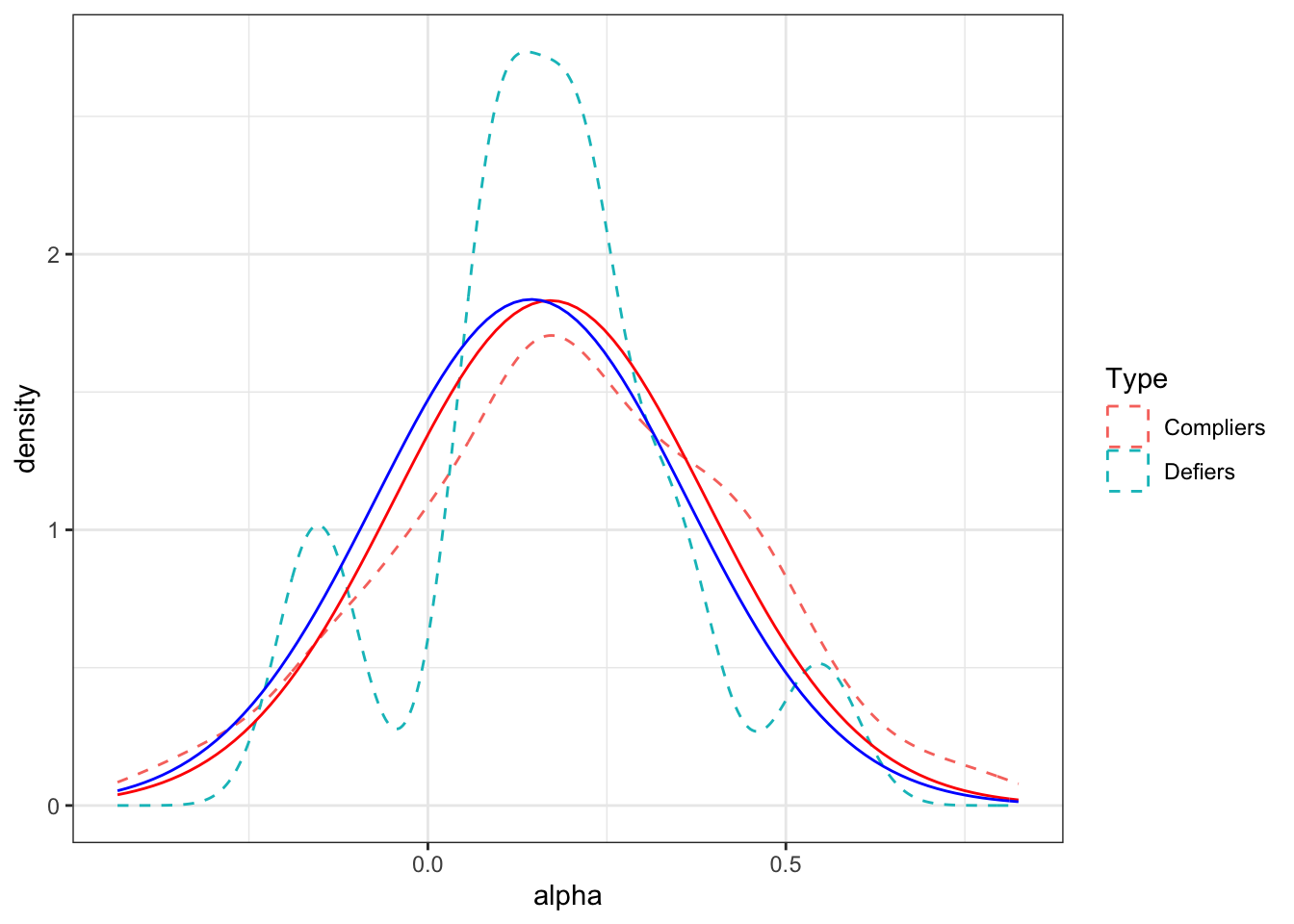

Figure 4.3: Distribution of treatment effects by Type in the sample (dashed line) and in the population (full line)

Figure 4.3 shows that the two distributions are actually very similar in our example. The distribution for the compliers is slightly above that for the defiers, meaning that the defiers should have lower expected outcomes in the population. Let us check that by computing the average outcomes of compliers and defiers both in the sample and in the population.

# sample means
mean.alpha.compliers.samp <- mean(alpha[C==1]) 
mean.alpha.defiers.samp <- mean(alpha[D==1]) 

# population means
mean.alpha.compliers.pop <- mtmvnorm(mean=mean.alpha.yBV,sigma=cov.alpha.yBV,lower=lower.cut.comp,upper=upper.cut.comp,doComputeVariance=FALSE)[[1]]
mean.alpha.defiers.pop <-  mtmvnorm(mean=mean.alpha.yBV,sigma=cov.alpha.yBV,lower=lower.cut.def,upper=upper.cut.def,doComputeVariance=FALSE)[[1]]

In the population, the average treatment effect for compliers is equal to 0.17 and the average treatment effect for defiers is equal to 0.14. In the sample, the average treatment effect for compliers is equal to 0.2 and the average treatment effect for defiers is equal to 0.16.

The difference between the treatment effect for compliers and defiers is a problem for the Wald estimator. Let’s look at how the Wald estimator behaves in the population (in order to avoid considerations due to sampling noise). By Theorem 3.10, the numerator of the Wald estimator is equal to the difference between the average treatment on compliers and the average treatment effect on defiers weighted by their respective proportions in the population. In order to be able to compute the Wald estimator, we need to compute the proportion of compliers and of defiers in the population. These proportions are equal to:

\[\begin{align*} \Pr(T_i=c) & = \Pr(\bar{y}< y_i^B+V_i\leq\bar{y}+\bar{\kappa}\cap\kappa_i=-\bar{\kappa}) \\ & = \Pr(\bar{y}< y_i^B+V_i\leq\bar{y}+\bar{\kappa})p_{\xi} \\ \Pr(T_i=d) & = \Pr(\bar{y}-\underline{\kappa}< y_i^B+V_i\leq\bar{y}\cap\kappa_i=\underline{\kappa}) \\ & = \Pr(\bar{y}-\underline{\kappa}< y_i^B+V_i\leq\bar{y})(1-p_{\xi}), \end{align*}\]

where the second equality follows from the fact that $\xi$ is independent from $y_i^B+V_i$ and uses the fact that $\Pr(A\cap B)=\Pr(A|B)\Pr(B)$. Since $y_i^B+V_i$ is normally distributed and we know its mean and variance, these proportions can be computed as:

\[\begin{align*} \Pr(T_i=c) & = p_{\xi}\left(\Phi\left(\frac{\bar{y}+\bar{\kappa}-\bar{\mu}}{\sqrt{(1+\gamma^2)\sigma^2_{\mu}+\sigma^2_U+\sigma^2_{\omega}}}\right) -\Phi\left(\frac{\bar{y}-\bar{\mu}}{\sqrt{(1+\gamma^2)\sigma^2_{\mu}+\sigma^2_U+\sigma^2_{\omega}}}\right)\right) \\ \Pr(T_i=d) & = (1-p_{\xi})\left(\Phi\left(\frac{\bar{y}-\bar{\mu}}{\sqrt{(1+\gamma^2)\sigma^2_{\mu}+\sigma^2_U+\sigma^2_{\omega}}}\right) -\Phi\left(\frac{\bar{y}-\underline{\kappa}-\bar{\mu}}{\sqrt{(1+\gamma^2)\sigma^2_{\mu}+\sigma^2_U+\sigma^2_{\omega}}}\right)\right). \end{align*}\]

Let’s write functions to compute these objects:

# proportion compliers
Prop.Comp <- function(param){
  first <- pnorm((log(param['barY'])+param['barkappa']-param['barmu'])/(sqrt((1+param['gamma']^2)*param['sigma2mu']+param['sigma2U']+param['sigma2omega'])))
  second <- pnorm((log(param['barY'])-param['barmu'])/(sqrt((1+param['gamma']^2)*param['sigma2mu']+param['sigma2U']+param['sigma2omega'])))
  return(param['pxi']*(first - second))  
}

# proportion defiers
Prop.Def <- function(param){
  first <- pnorm((log(param['barY'])-param['barmu'])/(sqrt((1+param['gamma']^2)*param['sigma2mu']+param['sigma2U']+param['sigma2omega'])))
  second <- pnorm((log(param['barY'])-param['underbarkappa']-param['barmu'])/(sqrt((1+param['gamma']^2)*param['sigma2mu']+param['sigma2U']+param['sigma2omega'])))
  return((1-param['pxi'])*(first - second))  
}

In our example, the proportion of compliers is equal to 0.33 and the proportion of defiers is equal to 0.01. As a consequence, the population value of the numerator of the Wald estimator is equal to 0.05. In the Wald estimator, this quantity is divided by the difference between the proportion of participants when $Z_i=1$ and when $Z_i=0$. We have already computed this quantity earlier, but it is nice to try to compute it in a different way using the types. The difference in the proportion of participants when $Z_i=1$ and when $Z_i=0$ is indeed equal to the difference in the proportion of compliers and the proportion of defiers. The difference between the proportion of compliers and the proportion of defiers is equal to 0.32, while the difference between the proportion of participants when $Z_i=1$ and when $Z_i=0$ is equal to 0.32. It is reassuring that we find the same thing (actually, full disclosure, I did not find the same thing at first, and this help me spot a mistake in the formulas for the proportions of participants: mistakes are normal and natural and that is how we learn and grow).

So we are now equipped to compute the value of the Wald estimator in the population in our model without monotonicity. It is equal to 0.172. In practice, the bias of the Wald estimator is rather small for the average treatment effect on the compliers (remember that it is equal to 0.171). In order to understand why, it is useful to see that the bias of the Wald estimator for the average treatment effect on the compliers is equal to:

\[\begin{align*} \esp{\Delta_i^Y|T_i=c}-\Delta^Y_{Wald} & = \esp{\Delta_i^Y|T_i=c} + (\esp{\Delta_i^Y|T_i=c}-\esp{\Delta_i^Y|T_i=d})\frac{\Pr(T_i=d)}{\Pr(T_i=c)-\Pr(T_i=d)}, \end{align*}\]

where the equality follows from Theorem 3.10 and some algebra. In the absence of Monotonicity, when the impact on defiers is smaller than the impact of compliers, the Wald estimator is baised upward for the effect on the compliers (as it happens in our example). In a model in which the effect of the treatment is larger on defiers than on compliers, the Wald estimator is biased downwards for the effect on compliers because defiers make the outcome of the control group seem too good. In the extreme, when $\esp{\Delta_i^Y|T_i=d}>\esp{\Delta_i^Y|T_i=c}(1+\frac{\Pr(T_i=c)-\Pr(T_i=d)}{\Pr(T_i=d)})$, the Wald estimator can be negative whereas the effects on compliers and on defiers are both positive. This happens when the effect on defiers is $1+\frac{\Pr(T_i=c)-\Pr(T_i=d)}{\Pr(T_i=d)}$ times larger than the effect on compliers. In our case, that means that the effect on defiers should be 26 times larger than the effect on compliers for the Wald estimator to be negative, that is to say the effect on defiers should be equal to 4.41, really much much much larger than the effect on compliers.

From there, we are going to explore three strategies in order to identify some true effect of the treatment using the Wald estimator:

The first strategy has been recently proposed by de Chaisemartin (2017). It is valid in a model without monotonicity.
The second strategy assumes that the heterogeneity in treatment effects is uncorrelated to the treatment.
The last strategy is due to Imbens and Angrist (1994) and assumes that Monotonicity holds.

Let’s review these solutions in turn.

4.1.2.1 Identification without Monotonicity

The approach delineated by de Chaisemartin (2017) does not assume away non-monotonicity. Clement instead assumes that we can divide the population of compliers in two-subpopulations: the compliers-defiers ($T_i=cd$) and the surviving-compliers ($T_i=sc$). The main assumption in Clement’s approach is that (i) the compliers-defiers are in the same proportion as the defiers and (ii) that the average effect of the treatment on the compliers defiers is equal as the average effect of the treatment on the defiers. These two assumptions can be formalized as follows:

Hypothesis 4.5 (Compliers-defiers) We assume that there exists as subpopulation of compliers that are in the same proportion as the defiers and for whom the average effect of the treatment is equal as the average effect of the treatment on the defiers:

\[\begin{align*} (T_i=c) & = (T_i=cd)\cup (T_i=sc) \\ \Pr(T_i=cd) & = \Pr(T_i=d) \\ \esp{Y^1_i-Y^0_i|T_i=cd} & = \esp{Y^1_i-Y^0_i|T_i=d}. \end{align*}\]

The first equation in Assumption 4.5 imposes that the compliers-defiers and the surviving-compliers are a partition of the population of compliers. From Assumption 4.5, we can prove the following theorem:

Theorem 4.1 (Identification of the effect on the surviving-compliers) Under Assumptions 4.1, 4.2, 4.3 and 4.5, the Wald estimator identifies the effect of the treatment on the surviving-compliers:

\[\begin{align*} \Delta^Y_{Wald} & = \Delta^Y_{sc}, \end{align*}\]

with:

\[\begin{align*} \Delta^Y_{Wald} & = \frac{\esp{Y_i|Z_i=1} - \esp{Y_i|Z_i=0}}{\Pr(D_i=1|Z_i=1)-\Pr(D_i=1|Z_i=0)}\\ \Delta^Y_{sc} & = \esp{Y^1_i-Y^0_i|T_i=sc}. \end{align*}\]

Proof. Under Assumptions 4.2 and 4.3, Theorems 3.10 and 3.12 imply that the numerator of the Wald estimator is equal to $\Delta^Y_{ITE}$ with:

\[\begin{align*} \Delta^Y_{ITE} & = \esp{Y_i^{1}-Y_i^{0}|T_i=c}\Pr(T_i=c)-\esp{Y_i^{1}-Y_i^{0}|T_i=d}\Pr(T_i=d). \end{align*}\]

Now, we have that the effect on compliers can be decomposed in the effect on surviving-compliers and the effect on compliers-defiers using the Law of Iterated Expectations and the fact that $T_i=sc \Rightarrow T_i=c$ and $T_i=cd \Rightarrow T_i=c$:

\[\begin{align*} \Delta^Y_{c} & = \esp{Y_i^{1}-Y_i^{0}|T_i=sc}\Pr(T_i=sc|T_i=c)+\esp{Y_i^{1}-Y_i^{0}|T_i=cd}\Pr(T_i=cd|T_i=c), \end{align*}\]

Now, using the fact that $\Pr(T_i=sc|T_i=c)\Pr(T_i=c)=\Pr(T_i=sc)$ and $\Pr(T_i=cd|T_i=c)\Pr(T_i=c)=\Pr(T_i=cd)$ (because $\Pr(A|B)\Pr(B)=\Pr(A\cap B)$ and $\Pr(A\cap B)=\Pr(A)$ if $A \Rightarrow B$), we have:

\[\begin{align*} \Delta^Y_{ITE} & = \esp{Y_i^{1}-Y_i^{0}|T_i=sc}\Pr(T_i=sc)\\ & \phantom{=}+\esp{Y_i^{1}-Y_i^{0}|T_i=cd}\Pr(T_i=cd)-\esp{Y_i^{1}-Y_i^{0}|T_i=d}\Pr(T_i=d). \end{align*}\]

The second part of the right-hand side of the above equation is equal to zero by virtue of Assumption 4.5. Now, under Assumptions 4.1, 4.2 and 4.3, we know, from the proof of Theorem 3.9, that $\Pr(D_i=1|Z_i=1)-\Pr(D_i=1|Z_i=0)=\Pr(T_i=c)-\Pr(T_i=d)$. Under Assumption 4.5, we have $\Pr(T_i=c)=\Pr((T_i=cd)\cup(T_i=sc))=\Pr(T_i=cd)+\Pr(T_i=sc)$. Replacing $\Pr(T_i=c)$ gives $\Pr(D_i=1|Z_i=1)-\Pr(D_i=1|Z_i=0)=\Pr(T_i=sc)$. Dividing $\Delta^Y_{ITE}$ by $\Pr(T_i=sc)$ gives the result.

Remark. de Chaisemartin (2017) shows in his Theorem 2.1 that the reciprocal of Theorem 4.1 is actually valid: if there exists surviving-compliers such that their effect is estimated by the Wald estimator and their proportion is equal to the denominator of the Wald estimator, then it has to be that there exists a sub-population of compliers-defiers that are in the same proportion as the defiers and have the same average treatment effect.

Example 4.7 Let us now see if the conditions in de Chaisemartin (2017) are verified in our numerical example.

I have bad news: they are not. It is not super easy to see why, but an intuitive explanation is that the average effect on the defiers in our model is taken conditional on $y^B_i+V_i\in]\bar{y}-\underline{\kappa},\bar{y}]$ while the effect on compliers is taken conditional on $y^B_i+V_i\in]\bar{y},\bar{y}+\bar{\kappa}]$. These two intervals do not overlap. Since the expected value of the treatment effect conditional on $y^B_i+V_i=v$ is monotonous in $v$ (because both variables come from a bivariate normal distribution), then all the effects on the defiers interval are either smaller or larger than all the effects on the compliers interval, making it impossible to find a sub-population of compliers that have the same average effect of the treatment as the defiers.

More formally, it is possible to prove this result by using the concept of Marginal Treatment Effect developed by Heckman and Vytlacil (1999). I might devote a specific section of the book to the MTE and its derivations. For now, I let it as a possibility.

What can we do then? Probably the best that we can do is to find $\kappa^*$ such that $\Pr(\bar{y}<y_i^B+V\leq\bar{y}+\kappa^*)p_{\xi}=\Pr(T_i=d)$, that is the value such that the interval of values of $y_i^B+V$ that are for compliers and closest to the interval for defiers and that contains the same proportion of compliers as there are defiers. This value is going to produce an average effect for compliers-defiers as close as possible to the average effect on defiers. It can be computed as follows:

\[\begin{align*} \kappa^* & = \bar{\mu}-\bar{y}+\sqrt{(1+\gamma^2)\sigma^2_{\mu}+\sigma^2_U+\sigma^2_{\omega}} \Phi^{-1}\Bigg(\Phi\left(\frac{\bar{y}-\bar{\mu}}{\sqrt{(1+\gamma^2)\sigma^2_{\mu}+\sigma^2_U+\sigma^2_{\omega}}}\right)\\ & \phantom{=}+\frac{1-p_{\xi}}{p_{\xi}}\left(\Phi\left(\frac{\bar{y}-\bar{\mu}}{\sqrt{(1+\gamma^2)\sigma^2_{\mu}+\sigma^2_U+\sigma^2_{\omega}}}\right)-\Phi\left(\frac{\bar{y}-\underline{\kappa}-\bar{\mu}}{\sqrt{(1+\gamma^2)\sigma^2_{\mu}+\sigma^2_U+\sigma^2_{\omega}}}\right)\right)\Bigg) \end{align*}\]

Let’s write functions to compute $\kappa^*$, the implied proportion of compliers-defiers and the average effect of the treatment on compliers-defiers and on surviving-compliers:

# kappa star
KappaStar <- function(param){
  prop.def <- Prop.Def(param)
  prop.below.bary <- pnorm((log(param['barY'])-param['barmu'])/(sqrt((1+param['gamma']^2)*param['sigma2mu']+param['sigma2U']+param['sigma2omega'])))
  st.dev.yB.V <- sqrt((1+param['gamma']^2)*param['sigma2mu']+param['sigma2U']+param['sigma2omega'])
  return(param['barmu']-log(param['barY'])+st.dev.yB.V*qnorm(prop.below.bary+prop.def/param['pxi']))
}

# proportion of compliers-defiers
Prop.Comp.Def <- function(param){
  first <- pnorm((log(param['barY'])+KappaStar(param)-param['barmu'])/(sqrt((1+param['gamma']^2)*param['sigma2mu']+param['sigma2U']+param['sigma2omega'])))
  second <- pnorm((log(param['barY'])-param['barmu'])/(sqrt((1+param['gamma']^2)*param['sigma2mu']+param['sigma2U']+param['sigma2omega'])))
  return(param['pxi']*(first - second))  
}

# mean impact on compliers-defiers
lower.cut.comp.def <- c(-Inf,log(param['barY']))
upper.cut.comp.def <- c(Inf,log(param['barY'])+KappaStar(param))
mean.alpha.comp.def.pop <- mtmvnorm(mean=mean.alpha.yBV,sigma=cov.alpha.yBV,lower=lower.cut.comp.def,upper=upper.cut.comp.def,doComputeVariance=FALSE)[[1]]

# mean impact on surviving compliers
lower.cut.surv.comp <- c(-Inf,log(param['barY'])+KappaStar(param))
upper.cut.surv.comp <- c(Inf,log(param['barY'])+param['barkappa'])

mean.alpha.surv.comp.pop <- mtmvnorm(mean=mean.alpha.yBV,sigma=cov.alpha.yBV,lower=lower.cut.surv.comp,upper=upper.cut.surv.comp,doComputeVariance=FALSE)[[1]]

The first have that $\kappa^*=$ 0.0452. For this value of $\kappa^*$, we have that $\Pr(T_i=cd)=$ 0.0128. As expected, this is very close to the proportion of compliers in the population: $\Pr(T_i=d)=$ 0.0128. Finally, the average treatment effect on the compliers-defiers is equal to: $\Delta^y_{cd}=$ 0.1457. As expected, but luckily enough, since it was absolutely not sure, it is very close to the to the average treatment effect on the defiers: $\Delta^y_{d}=$ 0.1445. So, in our model, Assumption 4.5 is almost satisfied, and so does Theorem 4.1. As a consequence, the Wald estimator is very close to the effect on the surviving-compliers. Indeed, the Wald estimator, in the population, is equal to $\Delta^y_{Wald}=$ 0.172156, while the average effect on surviving-compliers is equal to $\Delta^y_{sc}=$ 0.172108.

4.1.2.2 Identification under Independence of treatment effects

Another way to get around the issue of Non-Monotonicity is simply to assume away any meaningful role for treatment effect heterogeneity. One approach to that would simply be to assume that treatment effects are constant across individuals. I leave to the reader to prove that in that case, the Wald estimator would recover the treatment effect under only Independence and Exclusion Restriction. We are going to use a slightly more general approach here by assuming that treatment effect heterogeneity is unrelated to the reaction to the instrument:

Hypothesis 4.6 (Independent Treatment Effects) We assume that the treatment effect is independent from potential reactions to the instrument:

\[\begin{align*} \Delta^Y_i\Ind (D^1_i,D^0_i). \end{align*}\]

We can now prove that, under Assumption 4.6, the Wald estimator identifies the Average Treatment Effect (ATE), the average effect of the Treatment on the Treated (TT) and the average effect on compliers and on defiers. The first thing to know before we state the result is that, under Assumption 4.6, all these average treatment effects are equal to each other. This is a direct implication of the following lemma:

Lemma 4.1 (Independence of Treatment Effects from Types) Under Assumption 4.6, the treatment effect is independent from types:

\[\begin{align*} \Delta^Y_i\Ind T_i. \end{align*}\]

Proof. Lemma (4.2) in Dawid (1979) states that if $X \Ind Y|Z$ and $U$ is a function of $X$, then $U \Ind Y|Z$. Since $T_i$ is a function of $(D^1_i,D^0_i)$ under Assumption 4.6, Lemma 4.1 follows.

A direct corollary of Lemma 4.1 is:

Corollary 4.1 (Independence of Treatment Effects and Average Effects) Under Assumption 4.6, the Average Treatment Effect (ATE), the average effect of the Treatment on the Treated (TT) and the average effect on compliers and on defiers are all equal:

\[\begin{align*} \Delta^Y_{ATE} = \Delta^Y_{TT(1)} = \Delta^Y_{TT(0)} = \Delta^Y_{c} = \Delta^Y_{d}. \end{align*}\]

with: \[\begin{align*} \Delta^Y_{TT(z)} = \esp{Y_i^1-Y_i^0|D_i=1,Z_i=z}. \end{align*}\]

Proof. Using Lemma 4.1, we have that:

\[\begin{align*} \Delta^Y_{c} = \Delta^Y_{d} = \Delta^Y_{at} =\Delta^Y_{nt}. \end{align*}\]

Because $T_i$ is a partition, we have $\Delta^Y_{ATE}=\Delta^Y_{c}\Pr(T_i=c)+\Delta^Y_{d}\Pr(T_i=d)+\Delta^Y_{at}\Pr(T_i=at)+\Delta^Y_{nt}\Pr(T_i=nt)=\Delta^Y_{c}$ (since $\Pr(T_i=c)+\Pr(T_i=d)+\Pr(T_i=at)+\Pr(T_i=nt)=1$). Finally, we also have that $\Delta^Y_{TT(1)}=\Delta^Y_{c}\Pr(T_i=c|D_i=1,Z_i=1)+\Delta^Y_{at}\Pr(T_i=at|D_i=1,Z_i=1)=\Delta^Y_{c}$ and $\Delta^Y_{TT(0)}=\Delta^Y_{d}\Pr(T_i=d|D_i=1,Z_i=0)+\Delta^Y_{at}\Pr(T_i=at|D_i=1,Z_i=0)=\Delta^Y_{c}$, since $(D_i=1)\cap(Z_i=1)\Rightarrow (T_i=c)\cup(T_i=at)$ and $(D_i=1)\cap(Z_i=0)\Rightarrow (T_i=d)\cup(T_i=at)$.

We are now equipped to state the final result of this section:

Theorem 4.2 (Identification under Independent Treatment Effect) Under Assumptions 4.1, 4.2, 4.3 and 4.6, the Wald estimator identifies the average effect of the Treatment on the Treated:

\[\begin{align*} \Delta^Y_{Wald} & = \Delta^Y_{TT}. \end{align*}\]

Proof. Using the formula for the Wald estimator, we have, for the two components of its numerator:

\[\begin{align*} \esp{Y_i|Z_i=1} & = \esp{Y_i^0+(Y_i^1-Y_i^0)D_i|Z_i=1} \\ & = \esp{Y_i^0|Z_i=1}+\esp{\Delta^Y_i|D_i=1,Z_i=1}\Pr(D_i=1|Z_i=1)\\ & = \esp{Y_i^0|Z_i=1}+\Delta^Y_{TT(1)}\Pr(D_i=1|Z_i=1)\\ \esp{Y_i|Z_i=0} & = \esp{Y_i^0+(Y_i^1-Y_i^0)D_i|Z_i=0} \\ & = \esp{Y_i^0|Z_i=0}+\esp{\Delta^Y_i|D_i=0,Z_i=1}\Pr(D_i=1|Z_i=0)\\ & = \esp{Y_i^0|Z_i=0}+\Delta^Y_{TT(0)}\Pr(D_i=1|Z_i=0),\\ \end{align*}\]

where the first equalities use Assumption 4.2. Now, under Assumption 4.6, Corollary 4.1 implies that $\Delta^Y_{TT(0)}=\Delta^Y_{TT(1)}=\Delta^Y_{TT}$. We thus have that the numerator of the Wald estimator is equal to:

\[\begin{align*} \esp{Y_i|Z_i=1}-\esp{Y_i|Z_i=0} & = \Delta^Y_{TT}(\Pr(D_i=1|Z_i=1)-\Pr(D_i=1|Z_i=0))\\ & \phantom{=}+\esp{Y_i^0|Z_i=1}-\esp{Y_i^0|Z_i=0}. \end{align*}\]

Assumption 4.3 implies that $\esp{Y_i^0|Z_i=1}=\esp{Y_i^0|Z_i=0}$. Using Assumption 4.1 proves the result.

4.1.2.3 Identification under Monotonicity

The classical approach to identification using instrumental variables is due to Imbens and Angrist (1994) and Angrist, Imbens and Rubin (1996). It rests on Assumption 4.4 or Monotonicity that we are now familiar with, that requires that the effect of the instrument on treatment participation moves everyone in the same direction.

Remark. For the rest of the section, we will assume that $\forall i$, $D^1_i\geq D_i^0$. It is without loss of generality, since if the initial treatment does not comply with this requirement, you can simply redefine a new treatment equal to $-D_i$.

Under Monotonicity, there are no defiers. This is what the following lemma shows:

Lemma 4.2 Under Assumption 4.4, there are no defiers a.s.:

\[\begin{align*} \Pr(T_i=c) & = 0. \end{align*}\]

Proof. Under Assumption 4.4, $\forall i$, $D^1_i\geq D_i^0$. As a consequence, $\Pr(D^1_i < D_i^0)=0$. Since defiers are defined as $D^1_i < D_i^0$, the result follows.

In the absence of defiers, the Wald estimator identifies the average effect of the treatment on the compliers, also called the Local Average Treatment Effect:

Theorem 4.3 Under Assumptions 4.1, 4.2, 4.3 and 4.4, the Wald estimator identifies the average effect of the treatment on the compliers, also called the Local Average Treatment Effect:

\[\begin{align*} \Delta^Y_{Wald}& = \Delta^Y_{LATE}. \end{align*}\]

Proof. Using Theorem 3.9 directly proves the result.

Remark. The magic of the instrumental variables setting applies again. By moving the instrument, we are able to learn something about the causal effect of the treatment. Monotonicity is a very strong assumption though, as are Independence and Exclusion Restriction. They are very rarely met in practice. Even the case of RCTs with encouragement design, where Independence holds by design, might be affected by failures of Exclusion Restriction and/or Monotonicity.

Example 4.8 Let’s see how monotonicity works in our example.

First, we have to generate a model in which monotonicity holds. For that, we need to shut down heterogeneous reactions to the instrument. In practice, we are going to replace the participation equation in our model, which was characterized by a random coefficient, by the following one, which has a constant coefficient:

\[\begin{align*} D_i & = \uns{y_i^B-\bar{\kappa} Z_i + V_i\leq\bar{y}} \end{align*}\]

As a consequence, we have no more defiers and monotonicity holds. Let us now generate the data from the model with monotonicity:

set.seed(12345)
N <-1000
cov.eta.omega <- matrix(c(param["sigma2eta"],param["rhoetaomega"]*sqrt(param["sigma2eta"]*param["sigma2omega"]),param["rhoetaomega"]*sqrt(param["sigma2eta"]*param["sigma2omega"]),param["sigma2omega"]),ncol=2,nrow=2)
eta.omega <- as.data.frame(mvrnorm(N,c(0,0),cov.eta.omega))
colnames(eta.omega) <- c('eta','omega')
mu <- rnorm(N,param["barmu"],sqrt(param["sigma2mu"]))
UB <- rnorm(N,0,sqrt(param["sigma2U"]))
yB <- mu + UB 
YB <- exp(yB)
Ds <- rep(0,N)
Z <- rbinom(N,1,param["pZ"])
V <- param["gamma"]*(mu-param["barmu"])+eta.omega$omega
Ds[yB-param["barkappa"]*Z+V<=log(param["barY"])] <- 1 
epsilon <- rnorm(N,0,sqrt(param["sigma2epsilon"]))
U0 <- param["rho"]*UB + epsilon
y0 <- mu +  U0 + param["delta"]
alpha <- param["baralpha"]+  param["theta"]*mu + eta.omega$eta
y1 <- y0+alpha
Y0 <- exp(y0)
Y1 <- exp(y1)
y <- y1*Ds+y0*(1-Ds)
Y <- Y1*Ds+Y0*(1-Ds)

We can now define the types variable $T_i$:

D1 <- ifelse(yB-param["barkappa"]+V<=log(param["barY"]),1,0)
D0 <- ifelse(yB+V<=log(param["barY"]),1,0)
AT <- ifelse(D1==1 & D0==1,1,0)
NT <- ifelse(D1==0 & D0==0,1,0)
C <- ifelse(D1==1 & D0==0,1,0)
D <- ifelse(D1==0 & D0==1,1,0)
Type <- ifelse(AT==1,'a',
            ifelse(NT==1,'n',
                   ifelse(C==1,'c',
                          ifelse(D==1,'d',""))))

data.mono <- data.frame(cbind(Type,C,NT,AT,D1,D0,Y,y,Y1,Y0,y0,y1,yB,alpha,U0,eta.omega$eta,epsilon,Ds,Z,mu,UB))

The first thing we can check is that there are no defiers. For that, let’s count the number of individuals who have $T_i=1$. It is equal to 0.

One thing that helped me understand how the IV approach under monotonicity works is the following graph:

plot(yB[AT==1]+V[AT==1],y[AT==1],pch=1,xlim=c(5,11),ylim=c(5,11),xlab="yB+V",ylab="Outcomes")
points(yB[NT==1]+V[NT==1],y[NT==1],pch=1,col='blue')
points(yB[C==1 & Ds==1]+V[C==1 & Ds==1],y[C==1 & Ds==1],pch=1,col='red')
points(yB[C==1 & Ds==0]+V[C==1 & Ds==0],y[C==1 & Ds==0],pch=1,col='green')
abline(v=log(param["barY"]),col="red")
abline(v=log(param["barY"])+param['barkappa'],col="red")
text(x=c(log(param["barY"]),log(param["barY"])+param['barkappa']),y=c(5,5),labels=c(expression(bar('y')),expression(bar('y')+bar(kappa))),pos=c(2,4),col=c("red","red"))
legend(5,10.5,c('AT','NT','C|D=1','C|D=0'),pch=c(1,1,1,1),col=c("black",'blue',"red",'green'),ncol=1)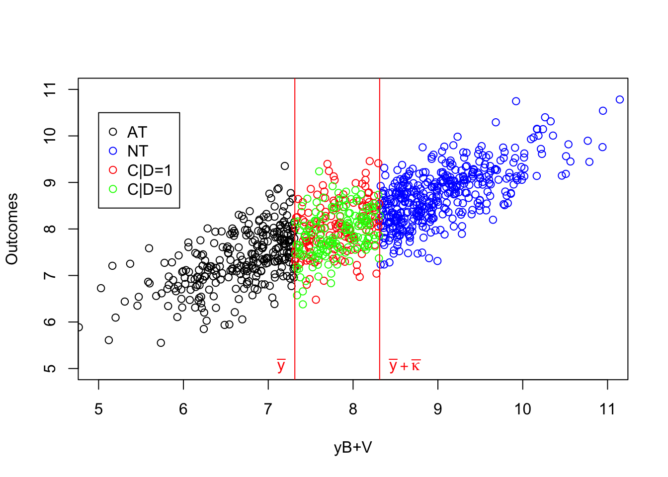

Figure 4.4: Types under Monotonicity

What 4.4 shows is that the IV acts as a randomized controlled trial among compliers. Within the population of compliers, whether one receives the treatment or not is as good as random. If we actually knew who the compliers were, we could directly estimate the effect of the treatment by comparing the outcomes of the treated compliers to the outcomes of the untreated compliers. Actually, this approach, applied in our sample, yields an estimated treatment effect on the compliers of 0.14, whereas the simple comparison of participants and non participants would give an estimate of -0.93. In our sample, the average effect of the treatment on compliers is actually equal to 0.18.

Let us finally check that Theorem 4.3 works in the population in our new model. We need to compute the various parts of the Wald estimator and the average effect of the treatment on the compliers. The key to understand the Wald estimator is to see that its numerator is composed of the difference between two means, with both means containing the average outcomes of always takers and never takers weighted by their respective proportions in the population, as shown in the proof of Theorem 4.3. These two means cancel out, leaving only the differences in the means of the compliers in and out of the treatment, weighted by their proportion in the population. The denominator of the Wald estimator simply provides an estimate of the proportion of compliers. In order to illustrate these intuitions in our example, I am going to use the formula for a truncated multivariate normal variable and the package tmvtnorm. The most important thing to notice here is that $(y^0_i,y^1_i,y_i^B+V_i) \sim \mathcal{N}\left(\bar{\mu}+\delta,\bar{\mu}(1+\theta)+\delta+\bar{\alpha},\bar{\mu},\mathbf{C}\right)$ with:

\[\begin{align*} \mathbf{C} &= \left(\begin{array}{ccc} \sigma^2_{\mu}+\rho^2\sigma^2_{U} +\sigma^2_{\epsilon} & (1+\theta)\sigma^2_{\mu}+\rho^2\sigma^2_U + \sigma^2_{\epsilon} & (1+\gamma)\sigma^2_{\mu}+\rho\sigma^2_U \\ (1+\theta)\sigma^2_{\mu}+\rho^2\sigma^2_U + \sigma^2_{\epsilon} & (1+\theta^2)\sigma^2_{\mu}+\rho^2\sigma^2_{U} +\sigma^2_{\epsilon} + \sigma^2_{\eta} & (1+\theta+\gamma)\sigma^2_{\mu}+\rho\sigma^2_U+\rho_{\eta,\omega}\sigma^2_{\eta}\sigma^2_{\omega} \\ (1+\gamma)\sigma^2_{\mu}+\rho\sigma^2_U & (1+\theta+\gamma)\sigma^2_{\mu}+\rho\sigma^2_U+\rho_{\eta,\omega}\sigma^2_{\eta}\sigma^2_{\omega} & (1+\gamma^2)\sigma^2_{\mu}+\sigma^2_U+\sigma^2_{\omega} \\ \end{array} \right) \end{align*}\]

We now simply have to derive the mean outcomes and proportions of each type in the population in order to form the Wald estimator. Let me first derive the joint distribution of the portential outcomes and the means and proportions of each type in the population.

mean.y0.y1.yBV <- c(param['barmu']+param['delta'],param['barmu']*(1+param['theta'])+param['delta']+param['baralpha'],param['barmu'])
cov.y0.y1.yBV <- matrix(c(param['sigma2mu']+param['rho']^2*param['sigma2U']+param['sigma2epsilon'],
                          (1+param['theta'])*param['sigma2mu']+param['rho']^2*param['sigma2U']+param['sigma2epsilon'],
                          (1+param['gamma'])*param['sigma2mu']+param['rho']*param['sigma2U'],
                          (1+param['theta'])*param['sigma2mu']+param['rho']^2*param['sigma2U']+param['sigma2epsilon'],
                          (1+param['theta']^2)*param['sigma2mu']+param['rho']^2*param['sigma2U']+param['sigma2epsilon']+param['sigma2eta'],
                          (1+param['theta']+param['gamma'])*param['sigma2mu']+param['rho']*param['sigma2U']+param['rhoetaomega']*param['sigma2eta']*param['sigma2omega'],
                          (1+param['gamma'])*param['sigma2mu']+param['rho']*param['sigma2U'],
                          (1+param['theta']+param['gamma'])*param['sigma2mu']+param['rho']*param['sigma2U']+param['rhoetaomega']*param['sigma2eta']*param['sigma2omega'],
                          (1+param['gamma']^2)*param['sigma2mu']+param['sigma2U']+param['sigma2omega']),3,3,byrow=TRUE)

# cuts
#always takers
lower.cut.at <- c(-Inf,-Inf,-Inf)
upper.cut.at <- c(Inf,Inf,log(param['barY']))
# compliers
lower.cut.comp <- c(-Inf,-Inf,log(param['barY']))
upper.cut.comp <- c(Inf,Inf,log(param['barY'])+param['barkappa'])
# never takers
lower.cut.nt <- c(-Inf,-Inf,log(param['barY'])+param['barkappa'])
upper.cut.nt <- c(Inf,Inf,Inf)

# means by types
#always takers
mean.y1.at.pop <- mtmvnorm(mean=mean.y0.y1.yBV,sigma=cov.y0.y1.yBV,lower=lower.cut.at,upper=upper.cut.at,doComputeVariance=FALSE)[[1]][[2]]
mean.y0.at.pop <- mtmvnorm(mean=mean.y0.y1.yBV,sigma=cov.y0.y1.yBV,lower=lower.cut.at,upper=upper.cut.at,doComputeVariance=FALSE)[[1]][[1]]
# never takers
mean.y1.nt.pop <- mtmvnorm(mean=mean.y0.y1.yBV,sigma=cov.y0.y1.yBV,lower=lower.cut.nt,upper=upper.cut.nt,doComputeVariance=FALSE)[[1]][[2]]
mean.y0.nt.pop <- mtmvnorm(mean=mean.y0.y1.yBV,sigma=cov.y0.y1.yBV,lower=lower.cut.nt,upper=upper.cut.nt,doComputeVariance=FALSE)[[1]][[1]]
#compliers
mean.y1.comp.pop <- mtmvnorm(mean=mean.y0.y1.yBV,sigma=cov.y0.y1.yBV,lower=lower.cut.comp,upper=upper.cut.comp,doComputeVariance=FALSE)[[1]][[2]]
mean.y0.comp.pop <- mtmvnorm(mean=mean.y0.y1.yBV,sigma=cov.y0.y1.yBV,lower=lower.cut.comp,upper=upper.cut.comp,doComputeVariance=FALSE)[[1]][[1]]

# Proportion of each types
# always takers
prop.at.pop <- ptmvnorm.marginal(log(param['barY']),n=3,mean=mean.y0.y1.yBV,sigma=cov.y0.y1.yBV)[[1]]
# never takers
prop.nt.pop <- 1-ptmvnorm.marginal(log(param['barY'])+param['barkappa'],n=3,mean=mean.y0.y1.yBV,sigma=cov.y0.y1.yBV)[[1]]
# compliers
prop.comp.pop <- ptmvnorm.marginal(log(param['barY'])+param['barkappa'],n=3,mean=mean.y0.y1.yBV,sigma=cov.y0.y1.yBV)[[1]]-ptmvnorm.marginal(log(param['barY']),n=3,mean=mean.y0.y1.yBV,sigma=cov.y0.y1.yBV)[[1]]

# LATE
late.pop <- mean.y1.comp.pop-mean.y0.comp.pop
late.prop.comp.pop <- late.pop*prop.comp.pop
# Wald
num.Wald.pop <- (mean.y1.comp.pop*prop.comp.pop+mean.y1.at.pop*prop.at.pop+mean.y0.nt.pop*prop.nt.pop-(mean.y0.comp.pop*prop.comp.pop+mean.y1.at.pop*prop.at.pop+mean.y0.nt.pop*prop.nt.pop))
denom.Wald.pop <- (prop.at.pop+prop.comp.pop-prop.at.pop)
Wald.pop <- num.Wald.pop/denom.Wald.pop

We are now equipped to compute the Wald estimator in the population. Before that, let us compute the LATE. We have $\Delta^Y_{LATE} =$ 0.179. The Wald estimator is equal to $\Delta^Y_{Wald} =$ 0.179. They are obviously equal. This is because the numerator of the Wald is equal to the product of the LATE multiplied by the proportion of compliers (which is equal to 0.066). This is because the outcomes of never takers and always takers cancel out on each separate term of the numerator of the Wald estimator. Indeed, we have that the numerator of the Wald estimator is equal to: 0.066.

4.1.3 Estimation

Estimation of the LATE under the IV assumptions closely follows the same steps that we have delineated in Section 3.4.2:

First stage regression of $D_i$ on $Z_i$: this estimates the impact of the instrument on participation into the program and estimates the proportion of compliers.
Reduced form regression of $Y_i$ on $Z_i$: this estimates the impact of the instrument on outcomes, a.k.a the ITE.
Structural regression of $Y_i$ on $D_i$ using $Z_i$ as an instrument, which estimates the LATE.

Let’s take these three steps in turn.

4.1.3.1 First stage regression

The first stage regression regresses $D_i$ on $Z_i$ and thus estimates the impact of the instrument on treatment participation, which is equal to the proportion of compliers. It can be run using the With/Without estimator or OLS (both are numerically equivalent as Lemma A.3 shows) or OLS conditioning on observed covariates.

Example 4.9 Let’s see how these three approaches fare in our example.

# WW first stage
WW.First.Stage.IV <- mean(Ds[Z==1])-mean(Ds[Z==0])
# Simple OLS
OLS.D.Z.IV <- lm(Ds~Z)
OLS.First.Stage.IV <- coef(OLS.D.Z.IV)[[2]]
# OLS conditioning on yB
OLS.D.Z.yB.IV <- lm(Ds~Z+yB)
OLSX.First.Stage.IV <- coef(OLS.D.Z.yB.IV)[[2]]

The WW estimator of the first stage impact of $Z_i$ on $D_i$ is equal to 0.374. The OLS estimator of the first stage impact of $Z_i$ on $D_i$ is equal to 0.374. The OLS estimator of the first stage impact of $Z_i$ on $D_i$ conditioning on $y^B_i$ is equal to 0.339. Remember that the true proportion of compliers in the population in our model is equal to 0.366.

4.1.3.2 Reduced form regression

The reduced form regression regresses $Y_i$ on $Z_i$ and thus estimates the impact of the instrument on outcomes, which is equal to the ITE. It can be run using the With/Without estimator or OLS (both are numerically equivalent as Lemma A.3 shows) or OLS conditioning on observed covariates.

Example 4.10 Let’s see how these three approaches fare in our example.

# WW reduced form
WW.Reduced.Form.IV <- mean(y[Z==1])-mean(y[Z==0])
# Simple OLS
OLS.y.Z.IV <- lm(y~Z)
OLS.Reduced.Form.IV <- coef(OLS.y.Z.IV)[[2]]
# OLS conditioning on yB
OLS.y.Z.yB.IV <- lm(y~Z+yB)
OLSX.Reduced.Form.IV <- coef(OLS.y.Z.yB.IV)[[2]]

The WW estimator of the reduced form impact of $Z_i$ on $y_i$ is equal to -0.029. The OLS estimator of the reduced form impact of $Z_i$ on $y_i$ is equal to -0.029. The OLS estimator of the reduced form impact of $Z_i$ on $y_i$ conditioning on $y^B_i$ is equal to 0.058. Remember that the true ITE in the population in our model is equal to 0.066.

4.1.3.3 Structural regression

The final step of the analysis is to estimate the impact of $D_i$ on $Y_i$ using $Z_i$ as an instrument. This can be done either by directly using the Wald estimator, by dividing the estimate of the reduced form by the result of the first stage, or by directly using the IV estimator (which is equivalent to the Wald estimator as Theorem 3.15 shows) or the IV estimator conditional on covariates.

Example 4.11 Let’s see how these four approaches fare in our example.

# Wald structural form
Wald.Structural.Form.IV <- (mean(y[Z==1])-mean(y[Z==0]))/(mean(Ds[Z==1])-mean(Ds[Z==0]))
# Simple IV
TSLS.y.D.Z.IV <- ivreg(y~Ds|Z)
TSLS.Structural.Form.IV <- coef(TSLS.y.D.Z.IV)[[2]]
# IV conditioning on yB
TSLS.y.D.Z.yB.IV <- ivreg(y~Ds+yB|Z+yB)
TSLSX.Structural.Form.IV <- coef(TSLS.y.D.Z.yB.IV)[[2]]

The Wald estimator of the LATE is equal to $\hat{\Delta}_{Wald}^{y}=$ -0.078. The IV estimator of the LATE is equal to $\hat{\Delta}_{IV}^{y}=$ -0.078, and is numerically identical to the Wald estimator, as expected. The IV estimator of the LATE conditioning on $y_i^B$ is equal to 0.172. Remember that the true LATE in the population in our model is equal to 0.179.

Remark. The last thing we might want to check is what the sampling noise of the IV estimator looks like and whether it is reduced by conditioning on observed covariates.

Example 4.12 Let’s see how sampling noise moves in our example.

Do it

4.1.4 Estimation of sampling noise

Remark. The framework we have seen here as been extended to multivalued instruments or treatments by several papers. Imbens and Angrist (1994) extend the framework to an ordered instrument. They show that the 2SLS estimator is a weighted average of LATEs for each values of the instrument, with positive weights summing to one. Angrist and Imbens (1995) extend the framework to he case where the treatment is an ordered discrete variable and there are multiple dichotomous instruments. They again show that the 2SLS estimator is a weighted average of LATEs with positive weights summing to one. Heckman and Vytlacil (1999) extend the framework to a case with a continuous instrument and show that one can the define a Marginal Treatment Effect (or MTE) that is equal to the effect of the treatment on individuals that have the same unobserved propensity to take the treatment. They show that the MTE can be identified by a limiting form of Wald estimator that they call a Local Instrumental Variable estimator. They also show that average treatment effect parameters such as TT, ATE and LATE are all weighted averages of the MTE, with positive weights summing to one. Under strong support conditions on the side of the instrument, one can thus in principle recover all treatment effect parameters with a continuous instrument.

Remark. One important concern with the first stage regression is that of weak instruments. When Assumption 4.1 does not hold and the impact on the instrument on take up is actually zero in the population, the Wald estimator is not well-defined.

Expand

4.2 Regression Discontinuity Designs

Regression Discontinuity Designs emerge in situations where there is a discontinuity in the probability of receiving the treatment. If there is also a discontinuity in outcomes, it is interpreted as the effect of the treatment. We distinguish two RD Designs:

Sharp Designs (the probability of receiving the treatment moves from 0 to 1 at the discontinuity,
Fuzzy Designs (the probability of receiving the treatment moves from values strictly between 0 and 1 at the discontinuity.

Let’s examine both of these configurations in turn.

4.2.1 Sharp Regression Discontinuity Designs

In Sharp Regression Discontinuity Designs, the following condition holds:

Hypothesis 4.7 (Sharp RDD Design) There exists a running variable $Z_i$ and a threshold $\bar{z}$ such that:

\[\begin{align*} D_i=\uns{Z_i\leq\bar{z}}. \end{align*}\]

Example 4.13 Let us illustrate this assumption in our example (it is easy since our basic selection rule has a discontinuous feature).

Let’s first choose parameter values and compute a function for the TT parameter:

param <- c(8,.5,.28,1500,0.9,0.01,0.05,0.05,0.05,0.1)
names(param) <- c("barmu","sigma2mu","sigma2U","barY","rho","theta","sigma2epsilon","sigma2eta","delta","baralpha")
delta.y.tt <- function(param){
  return(param["baralpha"]+param["theta"]*param["barmu"]-param["theta"]*((param["sigma2mu"]*dnorm((log(param["barY"])-param["barmu"])/(sqrt(param["sigma2mu"]+param["sigma2U"]))))/(sqrt(param["sigma2mu"]+param["sigma2U"])*pnorm((log(param["barY"])-param["barmu"])/(sqrt(param["sigma2mu"]+param["sigma2U"]))))))
}

Let us now simulate the data:

set.seed(1234)
N <-1000
mu <- rnorm(N,param["barmu"],sqrt(param["sigma2mu"]))
UB <- rnorm(N,0,sqrt(param["sigma2U"]))
yB <- mu + UB 
YB <- exp(yB)
Ds <- rep(0,N)
Ds[YB<=param["barY"]] <- 1 
epsilon <- rnorm(N,0,sqrt(param["sigma2epsilon"]))
eta<- rnorm(N,0,sqrt(param["sigma2eta"]))
U0 <- param["rho"]*UB + epsilon
y0 <- mu +  U0 + param["delta"]
alpha <- param["baralpha"]+  param["theta"]*mu + eta
y1 <- y0+alpha
Y0 <- exp(y0)
Y1 <- exp(y1)
y <- y1*Ds+y0*(1-Ds)
Y <- Y1*Ds+Y0*(1-Ds)

Let us now illustrate the resulting dataset:

par(mar=c(5,4,4,5))
plot(yB[Ds==0],y0[Ds==0],pch=1,xlim=c(5,11),ylim=c(5,11),xlab="yB",ylab="Outcomes")
points(yB[Ds==1],y[Ds==1],pch=3,col='blue')
abline(v=log(param["barY"]),col='red')
text(x=c(log(param["barY"])),y=c(5),labels=c(expression(bar('y'))),pos=c(2),col=c('red'))
legend(5,10.5,c('y0|D=0','y1|D=1','D'),pch=c(1,3,2),col=c('black','blue','red'),ncol=1)
par(new=TRUE)
plot(yB,Ds,pch=2,col='red',xlim=c(5,11),xaxt="n",yaxt="n",xlab="",ylab="")
axis(4)
mtext("D",side=4,line=3)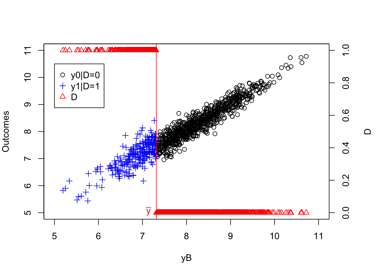

Figure 4.5: Sharp RDD Design

Figure 4.5 shows that there is a sharp decrease in treatment intake when moving above $y_i^B=\bar{y}$.

4.2.1.1 Identification

The main assumption we need on top of Assumption 4.7 is that outcomes are continuous around the threshold:

Hypothesis 4.8 (Continuity of Expected Potential Outcomes) For $d\in\left\{0,1\right\}$,

\[\begin{align*} \lim_{e\rightarrow 0^{+}}\esp{Y_i^d|Z_i=\bar{z}-e} & = \lim_{e\rightarrow 0^{+}}\esp{Y_i^d|Z_i=\bar{z}+e}. \end{align*}\]

Example 4.14 Let us see how this assumption works in our example.

We are going to use a linear conditional expectation to link $y^d_i$ and $y_i^B$, which is consistent since they are jointly normally distributed in our example. We fit the linear conditional expectation using OLS.

reg.ols.00 <- lm(y0[Ds==0]~yB[Ds==0])
reg.ols.01 <- lm(y0[Ds==1]~yB[Ds==1])
reg.ols.10 <- lm(y1[Ds==0]~yB[Ds==0])
reg.ols.11 <- lm(y1[Ds==1]~yB[Ds==1])

Let us now illustrate how these expectations look.

# plot for y1
plot(yB[Ds==0],y1[Ds==0],pch=3,xlim=c(5,11),ylim=c(5,11),col='red',xlab="yB",ylab="Outcomes")
points(yB[Ds==1],y1[Ds==1],pch=3)
points(yB[Ds==0],reg.ols.10$fitted.values,col='blue',pch=3)
points(yB[Ds==1],reg.ols.11$fitted.values,col='blue',pch=3)
abline(v=log(param["barY"]),col='red')
text(x=c(log(param["barY"])),y=c(5),labels=c(expression(bar('y'))),pos=c(2),col=c('red'))
legend(5,11,c('y1|D=0','y1|D=1','E[y1|yB]'),pch=c(3,3,3),col=c('red','black','blue'),ncol=2)

# plot for y0
plot(yB[Ds==0],y0[Ds==0],pch=1,xlim=c(5,11),ylim=c(5,11),col='black',xlab="yB",ylab="Outcomes")
points(yB[Ds==1],y0[Ds==1],pch=1,col='red')
points(yB[Ds==0],reg.ols.00$fitted.values,col='blue',pch=1)
points(yB[Ds==1],reg.ols.01$fitted.values,col='blue',pch=1)
abline(v=log(param["barY"]),col='red')
text(x=c(log(param["barY"])),y=c(5),labels=c(expression(bar('y'))),pos=c(2),col=c('red'))
legend(5,11,c('y0|D=0','y0|D=1','E[y0|yB]'),pch=c(1,1,1),col=c('black','red','blue'),ncol=2)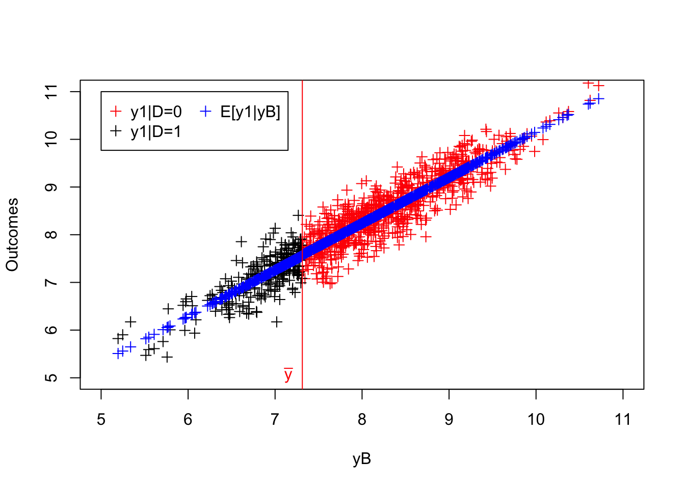

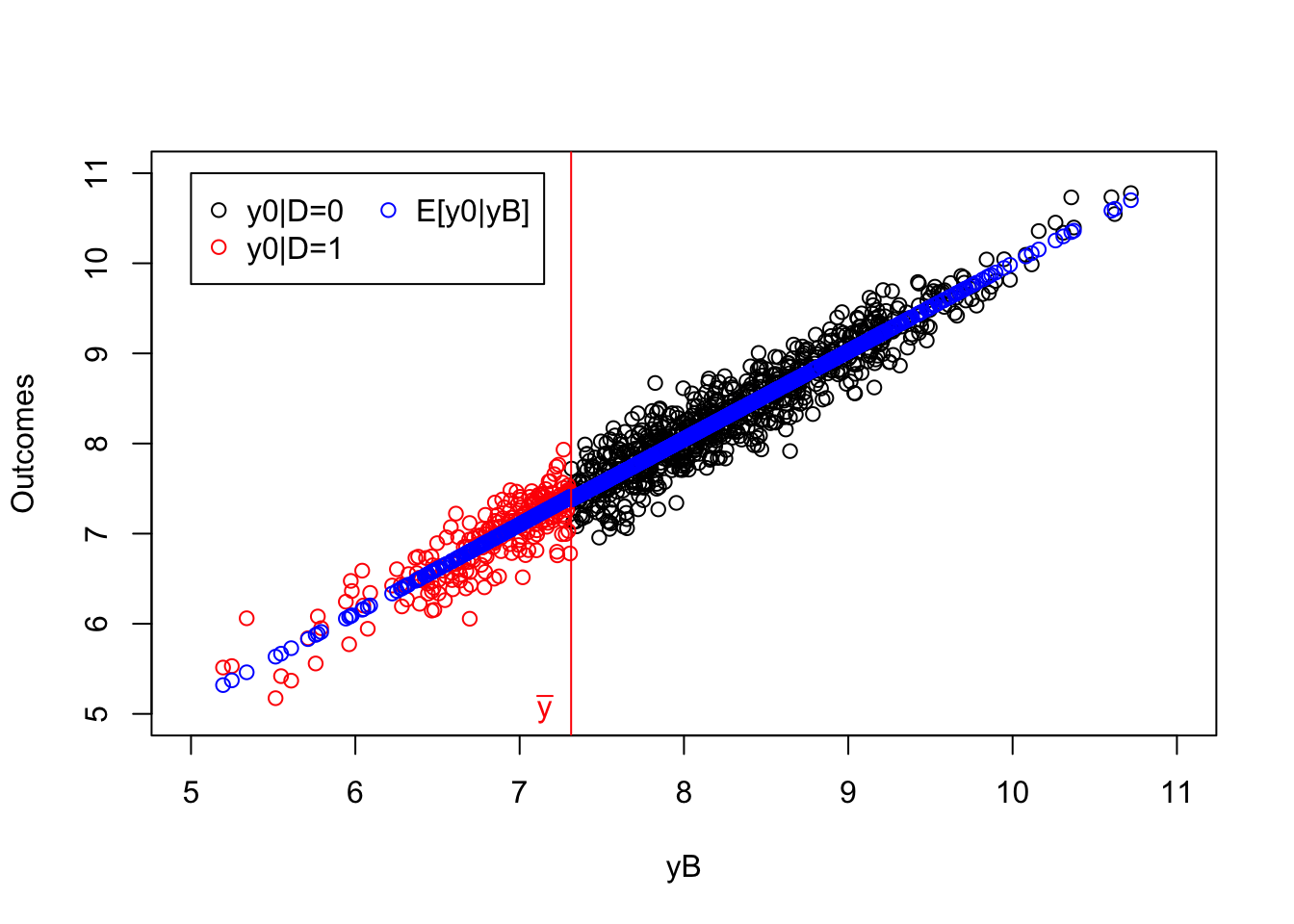
Figure 4.6: Continuity of potential outcomes

As we can see on Figure 4.6, at $\bar{y}$, both $\esp{y_i^1|y_i^B=y}$ and $\esp{y_i^0|y_i^B=y}$ are continuous.

Under Assumptions 4.7 and 4.8, we can prove identification of a local versino of the Treatment on the Treated parameter:

Theorem 4.4 (Identification in a Sharp RDD Design) Under Assumptions 4.7 and 4.8, the Treatment Effect on the Treated is identified at $Z_i=\bar{z}$:

\[\begin{align*} \Delta^Y_{TT}(\bar{z}) & = \lim_{e\rightarrow 0^{+}}\esp{Y_i|Z_i=\bar{z}-e}-\lim_{e\rightarrow 0^{+}}\esp{Y_i|Z_i=\bar{z}+e}, \end{align*}\]

where $\Delta^Y_{TT}(\bar{z})=\esp{\Delta^Y_i|Z_i=\bar{z}}$.

Proof. \[\begin{align*} \lim_{e\rightarrow 0^{+}}\esp{Y_i|Z_i=\bar{z}-e} -\lim_{e\rightarrow 0^{+}}\esp{Y_i|Z_i=\bar{z}+e} & = \lim_{e\rightarrow 0^{+}}\esp{Y^1_i|Z_i=\bar{z}-e} -\lim_{e\rightarrow 0^{+}}\esp{Y^0_i|Z_i=\bar{z}+e} \\ & = \esp{Y^1_i|Z_i=\bar{z}} - \esp{Y^0_i|Z_i=\bar{z}} \\ & = \esp{Y^1_i-Y^0_i|Z_i=\bar{z}} \\ & = \Delta^Y_{TT}(\bar{z}), \end{align*}\]

where the first equality uses Assumption 4.7 and the second equality uses Assumption 4.8.

Example 4.15 Let us try to illustrate how identification works in our numerical example.

plot(yB[Ds==0],y[Ds==0],pch=1,xlim=c(5,11),ylim=c(5,11),xlab="yB",ylab="Outcomes")
points(yB[Ds==1],y[Ds==1],pch=3)
points(yB[Ds==0],reg.ols.00$fitted.values,col='blue',pch=1)
points(yB[Ds==1],reg.ols.11$fitted.values,col='blue',pch=3)
abline(v=log(param["barY"]),col='black')
text(x=c(log(param["barY"])),y=c(5),labels=c(expression(bar('y'))),pos=c(2),col=c('black'))
legend(5,11,c('y0|D=0','y1|D=1',expression(hat('y0')),expression(hat('y1'))),pch=c(1,3,1,3),col=c('black','black','blue','blue'),ncol=2)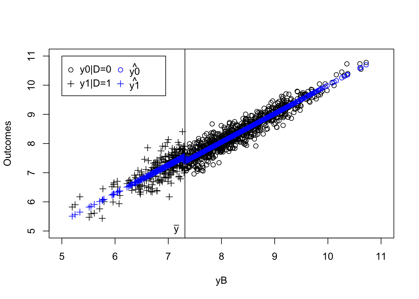

Figure 4.7: Identification in a sharp RDD design

On Figure 4.7, we can see a small decrease in the fitted lines just when we cross $y_i=\bar{y}$. This decrease is due to the positive effect of the treatment, since moving from above to below $\bar{y}$ swtiches the treatment on.

4.2.1.2 Estimation in a Sharp RD Design

For estimating the treatment effect in a Sharp RD Design, we can use OLS, if we are willing to assume that expected potential outcomes are a linear function of the running variable. This is obviously a huge assumption. In order to relax it, we can use non-parametric methods, and among them the ones that are unbiased when applied at a boundary of the parameter space. The best method in that case is the Local Linear Regression.

4.2.1.2.1 Estimation using OLS

Using OLS to estimate the treatment effect in a sharp RD Design works as follows. We fit two linear models, one on the left and one on the right of the discontinuity:

\[\begin{align*} \esp{Y_i|D_i=1,Z_i=z} & = \alpha_1+\beta_1z\\ \esp{Y_i|D_i=0,Z_i=z} & = \alpha_0+\beta_0z. \end{align*}\]

We then estimate the treatment effect by taking the difference in predicted outcomes at $Z_i=z$:

\[\begin{align*} \hat{\Delta}^Y_{TT}(z) & = \hatesp{Y_i|D_i=1,Z_i=z}-\hatesp{Y_i|D_i=0,Z_i=z}\\ & = \hat\alpha_1+\hat\beta_1z-\hat\alpha_0-\hat\beta_0z. \end{align*}\]

Example 4.16 Let’s see how this works in our example.

First, we need to compute the predicted values and the value of our estimated parameter:

# Predicted values
y0.bary.pred <- reg.ols.00$coef[[1]]+reg.ols.00$coef[[2]]*log(param['barY'])
y1.bary.pred <- reg.ols.11$coef[[1]]+reg.ols.11$coef[[2]]*log(param['barY'])
# estimated treatment effect
delta.y.rddols <- y1.bary.pred-y0.bary.pred

In order to be able to compare our estimate to the truth, let’s compute the true value of our target parameter:

\[\begin{align*} \Delta^y_{TT}(\bar{z}) & = \bar{\alpha} + \theta\bar{\mu}+\theta\frac{\sigma^2_{\mu}}{\sigma^2_{\mu}+\sigma^2_{U}}(\bar{y}-\bar{\mu}). \end{align*}\]

Let’s write a function to compute this formula:

delta.y.tt.z <- function(param){
  return(param["baralpha"]+param["theta"]*param["barmu"]+param["theta"]*(log(param["barY"])-param["barmu"])*param["sigma2mu"]/(param["sigma2mu"]+param["sigma2U"]))
}
delta.y.tt.z.pop <- delta.y.tt.z(param)

Our estimate of the treatment effect using OLS is thus 0.18 while the true value of our target parameter is 0.18.

4.2.1.2.2 Bias of the OLS RDD estimator when conditional expectations are nonlinear

The problem with the OLS approach to implement the RDD estimator is that it is highly dependent on the assumption that the conditional expectation functions $\esp{Y_i|D_i=d,Z_i=z}$ are linear. That might generate a strong functional form bias, as the following example shows.

Example 4.17 Let’s simulate some data in order to visualize the issue with OLS when the conditional expectation functions are non linear. In order to do that, we need to add some non linearity in the way potential outcomes are generated. We choose to make the equation for $y_i^0$ nonlinear in $y_i^B$:

\[\begin{align*} y_i^0 & = \mu_i+\delta+U_i^0 +\gamma*(y_i^B-\bar{y_i^B})^2. \end{align*}\]

Let’s choose some parameter values and simulate the data before seeing wht it looks like:

# parameters
param <- c(param,0.1,7.98)
names(param) <- c("barmu","sigma2mu","sigma2U","barY","rho","theta","sigma2epsilon","sigma2eta","delta","baralpha","gamma","baryB")

# simulations
set.seed(1234)
N <-1000
mu <- rnorm(N,param["barmu"],sqrt(param["sigma2mu"]))
UB <- rnorm(N,0,sqrt(param["sigma2U"]))
yB <- mu + UB 
YB <- exp(yB)
Ds <- rep(0,N)
Ds[YB<=param["barY"]] <- 1 
epsilon <- rnorm(N,0,sqrt(param["sigma2epsilon"]))
eta<- rnorm(N,0,sqrt(param["sigma2eta"]))
U0 <- param["rho"]*UB + epsilon
y0 <- mu +  U0 + param["delta"] + param["gamma"]*(yB-param["baryB"])^2
alpha <- param["baralpha"]+  param["theta"]*mu + eta
y1 <- y0+alpha
Y0 <- exp(y0)
Y1 <- exp(y1)
y <- y1*Ds+y0*(1-Ds)
Y <- Y1*Ds+Y0*(1-Ds)

# linear regressions
reg.ols.00 <- lm(y0[Ds==0]~yB[Ds==0])
reg.ols.01 <- lm(y0[Ds==1]~yB[Ds==1])
reg.ols.10 <- lm(y1[Ds==0]~yB[Ds==0])
reg.ols.11 <- lm(y1[Ds==1]~yB[Ds==1])

# predicted values and estimated treatment effect using lienar OLS
y0.bary.pred <- reg.ols.00$coef[[1]]+reg.ols.00$coef[[2]]*log(param['barY'])
y1.bary.pred <- reg.ols.11$coef[[1]]+reg.ols.11$coef[[2]]*log(param['barY'])
delta.y.rddols <- y1.bary.pred-y0.bary.pred

Let’s take a look at the data now:

plot(yB[Ds==0],y0[Ds==0],pch=1,xlim=c(5,11),ylim=c(5,11),xlab="yB",ylab="Outcomes")
points(yB[Ds==1],y1[Ds==1],pch=3,col='black')
points(yB[Ds==0],reg.ols.00$fitted.values,col='blue',pch=1)
points(yB[Ds==1],reg.ols.11$fitted.values,col='blue',pch=3)
abline(v=log(param["barY"]),col='black')
legend(5,11,c('y|D=0','y|D=1',expression(hat('y0')),expression(hat('y1'))),pch=c(1,3,1,3),col=c('black','black','blue','blue'),ncol=2)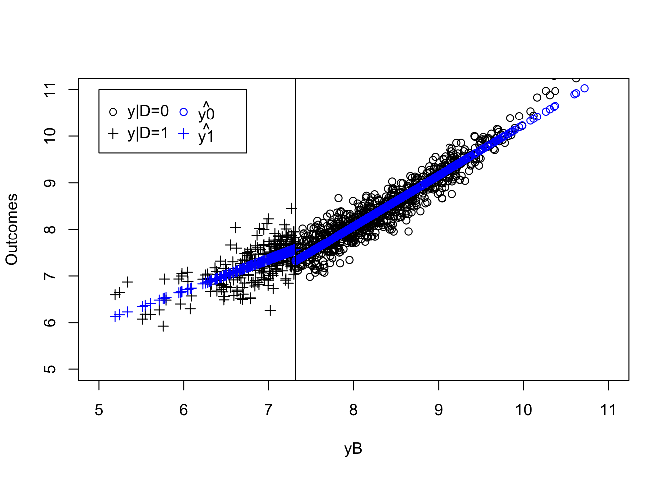

Figure 4.8: OLS estimates of sharp RDD with non linear conditional expectations

Our estimate of the treatment effect using OLS is now 0.25 while the true value of our target parameter is still 0.18. The reason wy the estimate is too large with respect to the truth is because the linear estimate of the conditional expectation $\hatesp{y_i^0|y_i^B=\bar{y}}$ is biased downwards: it should start curving upwards when approaching $\bar{y}$ but it does not, as we can see on Figure 4.8.

4.2.1.2.3 Estimation using Local Linear Regression

The reason the OLS RDD estimator fails when conditional expectations are nonlinear (as in Figure 4.8) is because the OLS estimate of the conditional expectation function is mispecified. What we need to replace OLS is an approach that is going to be well-specified under the assumption of continuous conditional expectations. We also want an estimator that behaves well (for example, is not biased) when operating at a boundary: note that we try to predict the value of the two conditional expectation functions just at the point after which they stop being defined. This second requirement is actually pretty harsh.

The most robust estimator that complies with these requirements is the Local Linear Regression estimator, or LLR. It is a basically just weighted OLS but only applied locally within a tiny window around the prediction point, with weights decreasing as they get further away from the prediction point. The weigths are generated by a kernel function. Which exact kernel function is used does not matter much in practice. What matters much more for LLR is the choice of the bandwidth, the width of the small window around the prediction point. Cross-validation (a form of leave-one-out assessment of goodness of fit) is generally used to choose the optimal bandwidth.

In short, the LLR RDD estimator works as follows:

Estimate $\hatesp{Y^1_i|D_i=1,Z_i=\bar{z}}$ using LLR on the treated side of the threshold.
Estimate $\hatesp{Y_i^0|D_i=0,Z_i=\bar{z}}$ using LLR on the untreated side of the threshold.
$\hat\Delta^{y}_{RDDLLR}=\hatesp{Y^1_i|D_i=1,Z_i=\bar{z}}-\hatesp{Y^0_i|D_i=0,Z_i=\bar{z}}$.
Bandwidth choice: use cross-validation on each side.

Example 4.18 Let’s see how all of this works in our example. First, let us code the LLR function and the cross validation function.

llr <- function(y,x,gridx,bw,kernel){
  if (kernel=='uniform'){
    K <- function(u){
      K.u <- 0
      if (abs(u)<=.5){K.u <- 1}
      return(K.u)
    }
  }
  if (kernel=='triangular'){
    K <- function(u){
      K.u <- 0
      if (abs(u)<=.5){K.u <- 2*(1-2*abs(u))}
      return(K.u)
    }
  }
  if (kernel=='epanechnikov'){
    K <- function(u){
      K.u <- 0
      if (abs(u)<=.5){K.u <- (3/2)*(1-4*u^2)}
      return(K.u)
    }
  }
  if (kernel=='quartic'){
    K <- function(u){
      K.u <- 0
      if (abs(u)<=.5){K.u <- (15/8)*(1-4*u^2)^2}
      return(K.u)
    }
  }
  if (kernel=='gaussian'){
    K <- function(u){
      return(exp(-0.5*u^2)/(sqrt(2*pi)))
    }
  }
  K.vec <- Vectorize(K)
  y0.hat <- rep(0,length(gridx))  
  for (i in (1:length(gridx))){
    x.i <- gridx[i]-x
    weights.i <- K.vec((x.i)/bw)
    ols.i <- lm(y~x.i,weights=weights.i)
    y0.hat[i] <- ols.i$coefficients[1]
  }
  return(y0.hat)
}

MSE.llr <- function(bw,y,D,x,kernel,d){
  MSE <- 0
  for (i in (1:length(y[D==d]))){
    MSE <- MSE + (y[D==d][i]-llr(y[D==d][-i],x[D==d][-i],x[D==d][i],bw=bw,kernel=kernel))^2
  }
  return(MSE)
}

We can now use these two functions to choose the optimal bandwidth on each side of the cut-off point:

kernel <- 'gaussian'
bw <- 0.5

MSE.grid <- seq(0.1,1,by=.1)
MSE.llr.0 <- sapply(MSE.grid,MSE.llr,y=y,D=Ds,x=yB,kernel=kernel,d=0)
MSE.llr.1 <- sapply(MSE.grid,MSE.llr,y=y,D=Ds,x=yB,kernel=kernel,d=1)
bw0 <- MSE.grid[MSE.llr.0==min(MSE.llr.0)]
bw1 <- MSE.grid[MSE.llr.1==min(MSE.llr.1)]

Let us see what the results of this computation look like:

par(mar=c(5,4,4,5))
plot(MSE.grid,MSE.llr.0,xlab='Bandwidth',ylab='MSE (y|D=0)')
legend(0.8,50,c('y|D=0','y|D=1'),pch=c(1,3),col=c('black','black'),ncol=1)
par(new=TRUE)
plot(MSE.grid,MSE.llr.1,pch=3,xaxt="n",yaxt="n",xlab="",ylab="")
axis(4)
mtext("MSE (y|D=1)",side=4,line=3)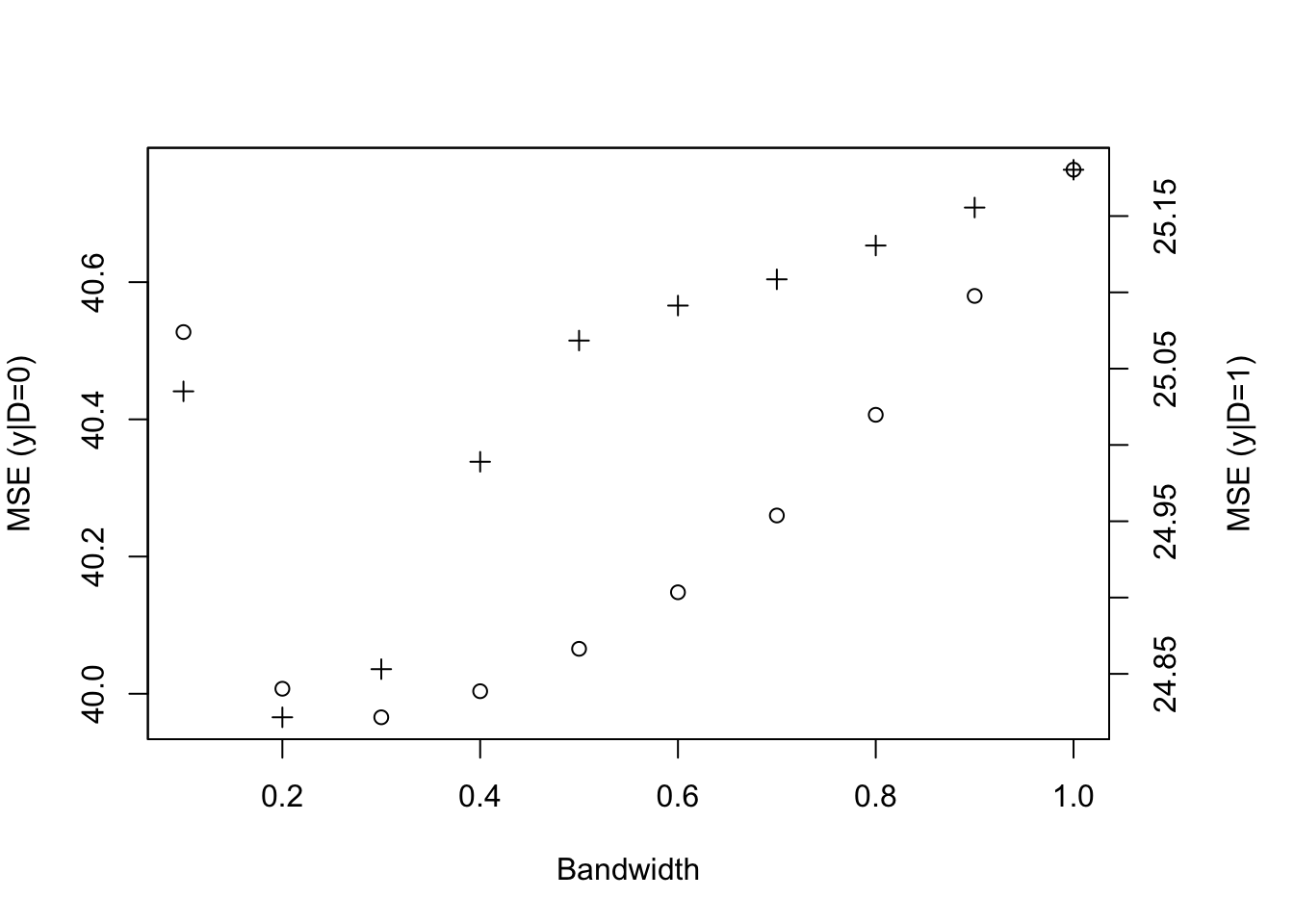

Figure 4.9: Cross Validation Results

As Figure 4.9 shows, the optimal bandwidth is equal to 0.3 on the right of the threshold and to 0.2 on the left.

We can now proceed with the estimation of the whole conditional expectations (in order to visualize them) and the estimated treatment effect using these optimal bandwidth levels:

# whole conditional expectations at each sample point
y0.llr <- llr(y[Ds==0],yB[Ds==0],yB[Ds==0],bw=bw0,kernel=kernel)    
y1.llr <- llr(y[Ds==1],yB[Ds==1],yB[Ds==1],bw=bw1,kernel=kernel)    

# estimation of the treatment effect
y0.bary.llr.pred <- llr(y[Ds==0],yB[Ds==0],c(log(param['barY'])),bw=bw0,kernel=kernel) 
y1.bary.llr.pred <- llr(y[Ds==1],yB[Ds==1],c(log(param['barY'])),bw=bw1,kernel=kernel)
delta.y.rdd.llr <- y1.bary.llr.pred-y0.bary.llr.pred

Let us plot the resulting estimates:

plot(yB[Ds==0],y[Ds==0],pch=1,xlim=c(5,11),ylim=c(5,11),xlab="yB",ylab="Outcomes")
points(yB[Ds==1],y[Ds==1],pch=3)
points(yB[Ds==0],y0.llr,col='blue',pch=1)
points(yB[Ds==1],y1.llr,col='blue',pch=3)
abline(v=log(param["barY"]),col='black')
text(x=c(log(param["barY"])),y=c(5),labels=c(expression(bar('y'))),pos=c(2),col=c('black'))
legend(5,11,c('y|D=0','y|D=1',expression(hat('y0')),expression(hat('y1'))),pch=c(1,3,1,3),col=c('black','black','blue','blue'),ncol=2)

Figure 4.10: LLR estimates of sharp RDD with non linear conditional expectations

Our estimate of the treatment effect using LLR is 0.19 while the true value of our target parameter is still 0.18. The reason why the LLR estimate is an improvement over the OLS estimate is because the LLR estimate of the conditional expectation $\hatesp{y_i^0|y_i^B=\bar{y}}$ curves upwards when approaching $\bar{y}$ as it should (as Figure 4.10 shows) while the linear prediction using OLS does not (see Figure 4.8).

Let us finally see how sampling noise moves that estimator around as sample size increases. I am first going to ignore the noise stemming from estimating the optimal bandwidth, because it increases computation time exponentially. I am going to stick with the bandwidths optimal for the test sample ($N=1000$). They are going to be too large for the large samples, and as a consequence, they are going to generate a biased estimator there. Let’s see how severe that is:

monte.carlo.rdd.llr.bw <- function(s,N,param,bw1,bw0,kernel){
  set.seed(s)
  mu <- rnorm(N,param["barmu"],sqrt(param["sigma2mu"]))
  UB <- rnorm(N,0,sqrt(param["sigma2U"]))
  yB <- mu + UB 
  YB <- exp(yB)
  Ds <- rep(0,N)
  Ds[YB<=param["barY"]] <- 1 
  epsilon <- rnorm(N,0,sqrt(param["sigma2epsilon"]))
  eta<- rnorm(N,0,sqrt(param["sigma2eta"]))
  U0 <- param["rho"]*UB + epsilon
  y0 <- mu +  U0 + param["delta"] + param["gamma"]*(yB-param["baryB"])^2
  alpha <- param["baralpha"]+  param["theta"]*mu + eta
  y1 <- y0+alpha
  Y0 <- exp(y0)
  Y1 <- exp(y1)
  y <- y1*Ds+y0*(1-Ds)
  Y <- Y1*Ds+Y0*(1-Ds)
  y0.bary.llr <- llr(y[Ds==0],yB[Ds==0],c(log(param['barY'])),bw=bw0,kernel=kernel)    
  y1.bary.llr <- llr(y[Ds==1],yB[Ds==1],c(log(param['barY'])),bw=bw1,kernel=kernel)    
  delta.y.rdd.llr <- y1.bary.llr-y0.bary.llr
  return(delta.y.rdd.llr)
}

simuls.rdd.llr.bw.N <- function(N,Nsim,param,bw0,bw1,kernel){
  simuls.rdd.llr.bw <- matrix(unlist(lapply(1:Nsim,monte.carlo.rdd.llr.bw,N=N,param=param,bw1=bw1,bw0=bw0,kernel=kernel)),nrow=Nsim,ncol=1,byrow=TRUE)
  colnames(simuls.rdd.llr.bw) <- c('RDD LLR')
  return(simuls.rdd.llr.bw)
}

sf.simuls.rdd.llr.bw.N <- function(N,Nsim,param,bw0,bw1,kernel){
  sfInit(parallel=TRUE,cpus=8)
  sfExport('llr','MSE.llr','param')
  sim <- matrix(unlist(sfLapply(1:Nsim,monte.carlo.rdd.llr.bw,N=N,param=param,bw1=bw1,bw0=bw0,kernel=kernel)),nrow=Nsim,ncol=1,byrow=TRUE)
  sfStop()
  colnames(sim) <- c('RDD LLR')
  return(sim)
}

Nsim <- 1000
#Nsim <- 10
N.sample <- c(100,1000,10000,100000)
#N.sample <- c(100,1000,10000)
#N.sample <- c(100,1000)
#N.sample <- c(1000)

simuls.rdd.llr.bw <- lapply(N.sample,sf.simuls.rdd.llr.bw.N,Nsim=Nsim,param=param,bw1=bw1,bw0=bw0,kernel=kernel)
names(simuls.rdd.llr.bw) <- N.sample

Let us now plot the results:

par(mfrow=c(2,2))
for (i in 1:length(simuls.rdd.llr.bw)){
  hist(simuls.rdd.llr.bw[[i]][,'RDD LLR'],breaks=30,main=paste('N=',as.character(N.sample[i])),xlab=expression(hat(Delta^yRDDLLR)),xlim=c(-0.15,0.55))
  abline(v=delta.y.tt.z(param),col="red")
}

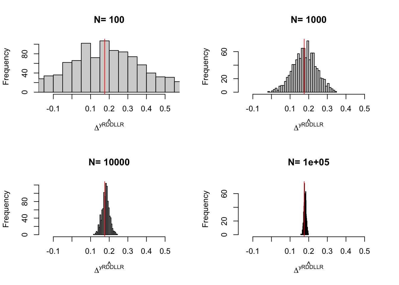
Figure 4.11: Distribution of the RDD LLR estimator over replications of samples of different sizes

As expected, there is a small downward bias for the sample sizes.

In order to see how much sampling noise estimates are affected by the computation of the optimal bandwidth, let’s run simulations including optimal bandwidth choice. Because of computational costs, I only run them for the smallest sample size for now.

monte.carlo.rdd.llr <- function(s,N,param){
  set.seed(s)
  mu <- rnorm(N,param["barmu"],sqrt(param["sigma2mu"]))
  UB <- rnorm(N,0,sqrt(param["sigma2U"]))
  yB <- mu + UB 
  YB <- exp(yB)
  Ds <- rep(0,N)
  Ds[YB<=param["barY"]] <- 1 
  epsilon <- rnorm(N,0,sqrt(param["sigma2epsilon"]))
  eta<- rnorm(N,0,sqrt(param["sigma2eta"]))
  U0 <- param["rho"]*UB + epsilon
  y0 <- mu +  U0 + param["delta"] + param["gamma"]*(yB-param["baryB"])^2
  alpha <- param["baralpha"]+  param["theta"]*mu + eta
  y1 <- y0+alpha
  Y0 <- exp(y0)
  Y1 <- exp(y1)
  y <- y1*Ds+y0*(1-Ds)
  Y <- Y1*Ds+Y0*(1-Ds)
  MSE.llr.0 <- sapply(MSE.grid,MSE.llr,y=y,D=Ds,x=yB,kernel=kernel,d=0)
  MSE.llr.1 <- sapply(MSE.grid,MSE.llr,y=y,D=Ds,x=yB,kernel=kernel,d=1)
  y0.bary.llr <- llr(y[Ds==0],yB[Ds==0],c(log(param['barY'])),bw=MSE.grid[MSE.llr.0==min(MSE.llr.0)],kernel=kernel)    
  y1.bary.llr <- llr(y[Ds==1],yB[Ds==1],c(log(param['barY'])),bw=MSE.grid[MSE.llr.1==min(MSE.llr.1)],kernel=kernel)    
  delta.y.rdd.llr <- y1.bary.llr-y0.bary.llr
  return(delta.y.rdd.llr)
}

simuls.rdd.llr.N <- function(N,Nsim,param){
  simuls.rdd.llr <- matrix(unlist(lapply(1:Nsim,monte.carlo.rdd.llr,N=N,param=param)),nrow=Nsim,ncol=1,byrow=TRUE)
  colnames(simuls.rdd.llr) <- c('RDD LLR')
  return(simuls.rdd.llr)
}

sf.simuls.rdd.llr.N <- function(N,Nsim,param){
  sfInit(parallel=TRUE,cpus=8)
  sfExport('llr','MSE.llr','param','MSE.grid','kernel','bw')
  sim <- matrix(unlist(sfLapply(1:Nsim,monte.carlo.rdd.llr,N=N,param=param)),nrow=Nsim,ncol=1,byrow=TRUE)
  sfStop()
  colnames(sim) <- c('RDD LLR')
  return(sim)
}

Nsim <- 1000
#Nsim <- 10
#N.sample <- c(100,1000,10000,100000)
#N.sample <- c(100,1000,10000)
#N.sample <- c(100,1000)
N.sample <- c(100)

simuls.rdd.llr <- lapply(N.sample,sf.simuls.rdd.llr.N,Nsim=Nsim,param=param)
names(simuls.rdd.llr) <- N.sample

Let’s plot the resulting estimate:

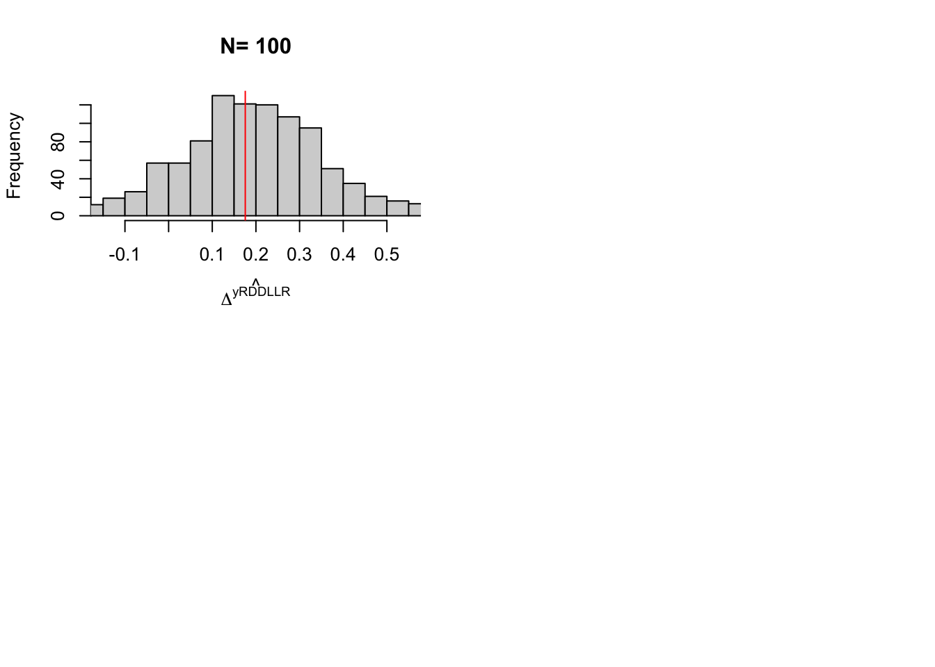
Figure 4.12: Distribution of the RDD LLR estimator over replications of samples of different sizes, with optimal bandwidth choice

The results are broadly comparable. For $N=100$, 99% sampling noise of LLR estimated by Monte Carlo simulations is 0.57 when keeping the bandwidth fixed while it is equal to 0.59 when the bandwidth is optimized at each run.

4.2.1.2.4 Simplified estimator of Lee and Lemieux

Imbens and Lemieux (2008) propose a simplified version of the RDD LLR estimator. $\hat{\delta}$ estimated by OLS on the sample of observations such as $\bar{z}-h\leq Z_i\leq\bar{z}+h$ is an estimate of $TT(z)$:

\[\begin{align*} Y_i & = \alpha + \beta (Z_i-\bar{z})(1-D_i) + \gamma(Z_i-\bar{z})D_i + \delta D_i + \epsilon_i \end{align*}\]

It is actually equal to the LLR estimate with uniform kernel and identical bandwidth on each side of the threshold.

Example 4.19 Lets run the simplified LLR estimator in our example.

bw <- 0.25
y.h <- y[log(param['barY'])-bw<yB & yB<log(param['barY'])+bw]
Ds.h <- Ds[log(param['barY'])-bw<yB & yB<log(param['barY'])+bw]
yB.l <- (yB[log(param['barY'])-bw<yB & yB<log(param['barY'])+bw]-log(param['barY']))*Ds[log(param['barY'])-bw<yB & yB<log(param['barY'])+bw]
yB.r <- (yB[log(param['barY'])-bw<yB & yB<log(param['barY'])+bw]-log(param['barY']))*(1-Ds[log(param['barY'])-bw<yB & yB<log(param['barY'])+bw])

reg.rdd.local.ols <- lm(y.h ~ Ds.h + yB.l + yB.r)
reg.rdd.local.ols$coef[2]

The estimated value of TT(z) by simplified LLR is 0.11 while the true value of our target parameter is still 0.18.

4.2.1.3 Estimating sampling noise

Several approaches are available to estimate sampling noise of the RDD LLR estimator in a sharp design:

Hahn, Todd and van der Klaauw (2001) derive general CLT results
Imbens and Lemieux (2008) simplify the CLT results and propose a plug-in estimator
Imbens and Lemieux (2008) propose to use the robust variance OLS estimator
We can always use the Bootstrap. It should be valid.

Let us first look at some CLT results:

Theorem 4.5 (Asymptotic Variance of the LLR Estimator in a Sharp RDD) Under standard assumptions, the variance of the simplified LLR Estimator in a Sharp Design can be approximated by:

\[\begin{align*} \var{\hat{\Delta}_{LLRRDD}} & \approx \frac{1}{Nh}\frac{4}{f_{Z}(\bar{z})}\left(\lim_{e\rightarrow 0^{\text{+}}}\var{Y_i|Z_i=\bar{z}-e}+\lim_{e\rightarrow 0^{\text{+}}}\var{Y_i|Z_i=\bar{z}+e}\right), \end{align*}\]

with $f_{Z}$ the density of $Z_i$.

Proof. See Hahn, Todd and van der Klaauw (2001) and Imbens and Lemieux (2008).

Example 4.20 Let’s see what happens when using the the robust variance estimator in the simplified LLR estimator proposed by Imbens and Lemieux (2008).

The estimated 99% sampling noise using this approach is 0.44 while the true 99% sampling noise of LLR estimated by Monte Carlo simulations is equal to 0.57.

4.2.2 Fuzzy Regression Discontinuity Designs

We say that a Regression Discontinuity Design is fuzzy when the probability of obtaining the treatment does not move from $0$ to $1$ when moving across the threshold of the running variable, but moves from some probability to a different one, when both are strictly positive and strictly smaller than one. This means that there is some event that discontinuously affects the enrollment of some people but not the enrollment of others. We thus are going to see compliers, always takers and never takers, as we did with Instrumental Variables. In this section, we are going to study the identification, estimation and estimation of sampling noise of treatment effects in the Fuzzy Regression Discontinuity Design.

4.2.2.1 Identification

The first assumption characterizing the Fuzzy Regression Discontinuity Design is the asumption that the probability of receiving treatment is discontinuous:

Hypothesis 4.9 (Fuzzy RDD Design) There exists a running variable $Z_i$ and a threshold $\bar{z}$ such that:

\[\begin{align*} \lim_{e\rightarrow 0^{+}}\Pr(D_i=1|Z_i=\bar{z}-e) & \neq \lim_{e\rightarrow 0^{+}}\Pr(D_i=1|Z_i=\bar{z}+e). \end{align*}\]

Example 4.21 Let’s see how this plays in our example. Let’s first simulate some data:

\[\begin{align*} y_i^1 & = y_i^0+\bar{\alpha}+\theta\mu_i+\eta_i \\ y_i^0 & = \mu_i+\delta+U_i^0+\gamma(y_i^B-\bar{y})^2 \\ U_i^0 & = \rho U_i^B+\epsilon_i \\ y_i^B & =\mu_i+U_i^B \\ U_i^B & \sim\mathcal{N}(0,\sigma^2_{U}) \\ D_i & = \uns{y_i^B\leq\bar{y} \land V_i\leq\kappa \lor y_i^B>\bar{y} \land V_i>\kappa} \\ (\eta_i,\omega_i,V_i) & \sim\mathcal{N}(0,0,0,\sigma^2_{\eta},\sigma^2_{\omega},\sigma^2_{\mu}+\sigma^2_{U},0,0,0). \end{align*}\]

param <- c(param,1)
names(param)[[length(param)]] <- "kappa"
N <- 1000
set.seed(123)
mu <- rnorm(N,param["barmu"],sqrt(param["sigma2mu"]))
UB <- rnorm(N,0,sqrt(param["sigma2U"]))
yB <- mu + UB 
YB <- exp(yB)
Ds <- rep(0,N)
V <- rnorm(N,0,sqrt(param["sigma2mu"]+param["sigma2U"]))
Ds[((yB<=log(param["barY"])) & (V<=param["kappa"])) | ((yB>log(param["barY"])) & (V>param["kappa"])) ] <- 1 
epsilon <- rnorm(N,0,sqrt(param["sigma2epsilon"]))
eta<- rnorm(N,0,sqrt(param["sigma2eta"]))
U0 <- param["rho"]*UB + epsilon
y0 <- mu +  U0 + param["delta"] + param["gamma"]*(yB-param["baryB"])^2
alpha <- param["baralpha"]+  param["theta"]*mu + eta
y1 <- y0+alpha
Y0 <- exp(y0)
Y1 <- exp(y1)
y <- y1*Ds+y0*(1-Ds)
Y <- Y1*Ds+Y0*(1-Ds)

Let us now plot the corresponding data:

par(mar=c(5,4,4,5))
plot(yB[Ds==0],y0[Ds==0],pch=1,xlim=c(5,11),ylim=c(5,11),xlab="yB",ylab="Outcomes")
points(yB[Ds==1],y[Ds==1],pch=3,col='black')
abline(v=log(param["barY"]),col='red')
legend(5,10.5,c('y0|D=0','y1|D=1','D'),pch=c(1,3,2),col=c('black','black','red'),ncol=1)
par(new=TRUE)
plot(yB,Ds,pch=2,col='red',xlim=c(5,11),xaxt="n",yaxt="n",xlab="",ylab="")
axis(4)
mtext("D",side=4,line=3)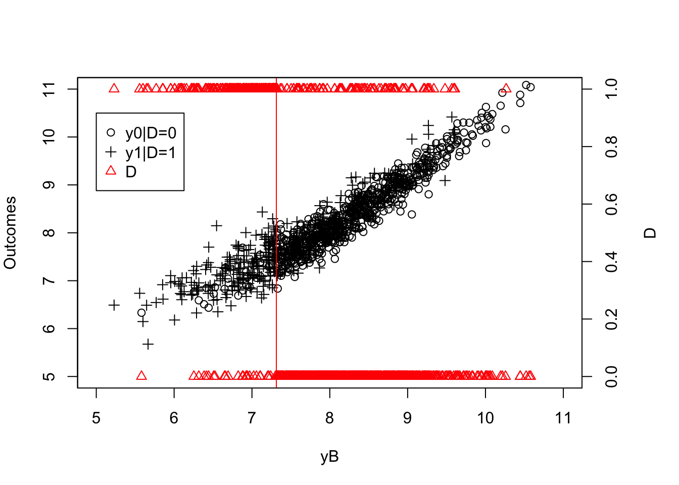

Figure 4.13: Fuzzy RDD

As you can see on Figure 4.13, there are untreated individuals below $\bar{y}$ and treated individual above $\bar{y}$. This is why the design is not sharp. But Figure 4.13 fails to convey that the design still exhibits a discontinuity in the proportion of treated. In order to see it, we need to compute an estimate of the probability of being treated conditional on the running variable ($y_i^B$): $\Pr(D_i=1|y_i^B=y)$. It turns out that this quantity is simply the expected value of $D_i$ conditional on $y_i^B$. We’ve just learned a cool way to estimate a conditional expectation: Local Linear Regression. Let’s put it to work, using $D_i$ as the outcome variable now:

kernel <- 'gaussian'
MSE.grid <- seq(0.1,1,by=.1)
# the instrument in our case is the position relative to the threshoold (or side, hence S)
S <- rep(0,length(yB))
S[yB<=log(param['barY'])] <- 1

# computing optimal bandwidth using Cross Validation
MSE.pr.llr.0 <- sapply(MSE.grid,MSE.llr,y=Ds,D=S,x=yB,kernel=kernel,d=0)
MSE.pr.llr.1 <- sapply(MSE.grid,MSE.llr,y=Ds,D=S,x=yB,kernel=kernel,d=1)
bwD0 <- MSE.grid[MSE.pr.llr.0==min(MSE.pr.llr.0)]
bwD1 <- MSE.grid[MSE.pr.llr.1==min(MSE.pr.llr.1)]

# LLR estoimate of conditional expectation of D on yB
Pr.D0.llr <- llr(Ds[S==0],yB[S==0],yB[S==0],bw=bwD0,kernel=kernel)    
Pr.D1.llr <- llr(Ds[S==1],yB[S==1],yB[S==1],bw=bwD1,kernel=kernel)

Let’s now plot the resulting estimate:

par(mar=c(5,4,4,5))
plot(yB[Ds==0],y0[Ds==0],pch=1,xlim=c(5,11),ylim=c(5,11),xlab="yB",ylab="Outcomes")
points(yB[Ds==1],y[Ds==1],pch=3,col='black')
abline(v=log(param["barY"]),col='red')
legend(5,10.5,c('y0|D=0','y1|D=1','D','Pr(D=1|S=1,yB)','Pr(D=1|S=0,yB)'),pch=c(1,3,2,3,1),col=c('black','black','red','red','red'),ncol=1)
par(new=TRUE)
plot(yB,Ds,pch=2,col='red',xlim=c(5,11),xaxt="n",yaxt="n",xlab="",ylab="")
points(yB[S==0],Pr.D0.llr,col='red')
points(yB[S==1],Pr.D1.llr,col='red',pch=3)
axis(4)
mtext("D",side=4,line=3)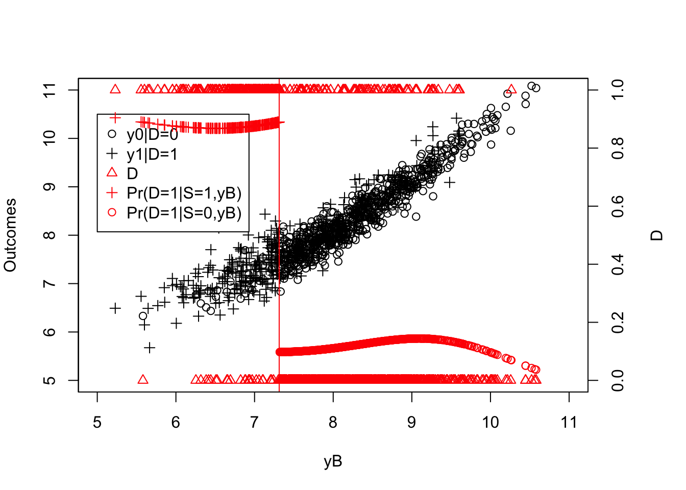

Figure 4.14: Fuzzy RDD with probability of being treated as a function of the running variable

Figure 4.13 now clearly shows that the probability of receiving the treatment decreases discontinuously when crossing the threshold $\bar{y}$. The decrease is not a move from $1$ to $0$ and hence is a clear case of a Fuzzy Regression Discontinuity Design.

Identification in a Fuzzy Regression Discontinuity Design proceeds along the same lines as with Instrumental Variables: either we assume that treatment effects are somewhat independent from Types or we impose that there are no defiers (though some more options are feasible, as we saw in the section on Instrumental Variables).

4.2.2.1.1 Identification under Independence of treatment effects from Types

Let us first define the types in a Fuzzy Regression Discontinuity Design. For that, we define $D_i(z)$ as the potential outcome of individual $i$ when $Z_i=z$. We have (as seems natural now) four possible types of individuals depending on how they react when exogenously moved from one side of the threshold to the other:

Always takers ($T^{\bar{z}}_i=a$) are such that $\lim_{z\rightarrow \bar{z}^+}D_i(z)=\lim_{z\rightarrow \bar{z}^-}D_i(z)=1$.
Never takers ($T^{\bar{z}}_i=n$) are such that $\lim_{z\rightarrow \bar{z}^+}D_i(z)=\lim_{z\rightarrow \bar{z}^-}D_i(z)=0$.
Compliers ($T^{\bar{z}}_i=c$) are such that $\lim_{z\rightarrow \bar{z}^+}D_i(z)-\lim_{z\rightarrow \bar{z}^-}D_i(z)=1$.
Defiers ($T^{\bar{z}}_i=d$) are such that $\lim_{z\rightarrow \bar{z}^+}D_i(z)-\lim_{z\rightarrow \bar{z}^-}D_i(z)=-1$.

We can now encode the assumption of independent treatment effects:

Hypothesis 4.10 (Independence of Treatment Effects from Types) We assume that treatment effects are independent of Types at the discontinuity:

\[\begin{align*} \Delta^Y_i\Ind T^{\bar{z}}_i|Z_i=z. \end{align*}\]

We are now equipped to prove identification in the Fuzzy Regression Discontinuity Design under Independence of Treatment Effects from Types:

Theorem 4.6 (Identification of TT(z) in Fuzzy RDD under Independence) Under Assumptions 4.8 and 4.10, we have:

\[\begin{align*} \Delta^Y_{RDDWALD} & = \Delta^Y_{TT}(z), \end{align*}\]

with

\[\begin{align*} \Delta^Y_{RDDWALD} & = \frac{\lim_{e\rightarrow 0^{+}}\esp{Y_i|Z_i=\bar{z}-e} - \lim_{e\rightarrow 0^{+}}\esp{Y_i|Z_i=\bar{z}+e}} {\lim_{e\rightarrow 0^{+}}\Pr(D_i=1|Z_i=\bar{z}-e) - \lim_{e\rightarrow 0^{+}}\Pr(D_i=1|Z_i=\bar{z}+e)} \end{align*}\]

Proof. Using the switching equation and Assumption 4.8, we can decompose the numerator of the Local Wald estimator as follows:

\[\begin{align*} \lim_{z\rightarrow \bar{z}^+}\esp{Y_i|Z_i=z}&=\esp{Y_i^1|Z_i=\bar{z},T^{\bar{z}}_i=a}\Pr(T_i=a|Z_i=\bar{z})\\ & \phantom{=}+\esp{Y_i^1|Z_i=\bar{z},T^{\bar{z}}_i=c}\Pr(T_i=c|Z_i=\bar{z})\\ & \phantom{=}+\esp{Y_i^0|Z_i=\bar{z},T^{\bar{z}}_i=d}\Pr(T_i=d|Z_i=\bar{z})\\ & \phantom{=}+\esp{Y_i^0|Z_i=\bar{z},T^{\bar{z}}_i=n}\Pr(T_i=n|Z_i=\bar{z})\\ \lim_{z\rightarrow \bar{z}^-}\esp{Y_i|Z_i=z}&=\esp{Y_i^1|Z_i=\bar{z},T^{\bar{z}}_i=a}\Pr(T_i=a|Z_i=\bar{z})\\ & \phantom{=}+\esp{Y_i^0|Z_i=\bar{z},T^{\bar{z}}_i=c}\Pr(T_i=c|Z_i=\bar{z})\\ & \phantom{=}+\esp{Y_i^1|Z_i=\bar{z},T^{\bar{z}}_i=d}\Pr(T_i=d|Z_i=\bar{z})\\ & \phantom{=}+\esp{Y_i^0|Z_i=\bar{z},T^{\bar{z}}_i=n}\Pr(T_i=n|Z_i=\bar{z})\\ N_{\bar{z}}&= \lim_{e\rightarrow 0^{+}}\esp{Y_i|Z_i=\bar{z}-e}- \lim_{e\rightarrow 0^{+}}\esp{Y_i|Z_i=\bar{z}+e}\\ & = \esp{Y_i^1-Y_i^0|Z_i=\bar{z},T^{\bar{z}}_i=c}\Pr(T_i=c|Z_i=\bar{z})\\ & \phantom{=}-\esp{Y_i^1-Y_i^0|Z_i=\bar{z},T^{\bar{z}}_i=d}\Pr(T_i=d|Z_i=\bar{z}) \end{align*}\]

We also have that the denominator of the Local Wald estimator is equal to:

\[\begin{align*} D_{\bar{z}}& =\lim_{z\rightarrow \bar{z}^+}\Pr(D_i=1|Z_i=z)-\lim_{z\rightarrow \bar{z}^-}\Pr(D_i=1|Z_i=z)\\ & = \lim_{z\rightarrow \bar{z}^+}\left(\Pr(T_i^z=a|Z_i=z)+\Pr(T_i^z=c|Z_i=z)\right)\\ & \phantom{=}-\lim_{z\rightarrow \bar{z}^-}\left(\Pr(T_i^z=a|Z_i=z)+\Pr(T_i^z=d|Z_i=z)\right)\\ & = \Pr(T_i^{\bar{z}}=c|Z_i=\bar{z})-\Pr(T_i^{\bar{z}}=d|Z_i=\bar{z}) \end{align*}\]

Under Assumption 4.10, we have that $\esp{Y_i^1-Y_i^0|Z_i=\bar{z},T^{\bar{z}}_i=c}=\esp{Y_i^1-Y_i^0|Z_i=\bar{z},T^{\bar{z}}_i=d}=\esp{Y_i^1-Y_i^0|Z_i=\bar{z}}$. This proves the result.

4.2.2.1.2 Identification under Monotonicity

We can weaken Assumption 4.10 and allow for treatment effects correlated with types (which seems highly likely) if we are willing to make stronger assumptions on the distribution of types. As we have seen before with Instrumental Variables, assuming away defiers enables the identification of a Local Average Treatment Effect. Let’s see how this works:

Hypothesis 4.11 (Monotonicity in a Fuzzy Regression Discontinuity Design) $D_i(z)$ is non-decreasing at $z=\bar{z}$ (or $\Pr(T^{\bar{z}}_i=d|Z_i=\bar{z})=0$).

We can now prove identification of the local average treatment effect:

Theorem 4.7 (Identification of TT(z) in Fuzzy RDD under Monotonicity) Under Assumptions 4.8 and 4.11, we have:

\[\begin{align*} \Delta^Y_{RDDWALD} & = \Delta^Y_{LATE}(z), \end{align*}\]

with

\[\begin{align*} \Delta^Y_{LATE}(z) & = \esp{y_i^1-Y_i^0|T_i^{\bar{z}}=c,Z_i=\bar{z}}. \end{align*}\]

Proof. The proof essentially follows the proof of Theorem 4.6 up to its penultimate step. Under Assumption 4.11, we have that $\Pr(T^{\bar{z}}_i=d|Z_i=\bar{z})=0$. This proves the result.

4.2.2.2 Estimation

For estimation, we can either use the Local Linear Regression Wald estimator or use a simplified version proposed by Imbens and Lemieux (2008). Let’s see how both of them work in practice.

4.2.2.2.1 Estimation using Local Linear Regression

The Wald LLR estimator can be formed as follows, with $S_i=1$ when $Z_i\geq\bar{z}$ and $S_i=0$ when $Z_i<\bar{z}$ (in the case where $\lim_{e\rightarrow 0^{+}}\Pr(D_i=1|Z_i=\bar{z}-e) < \lim_{e\rightarrow 0^{+}}\Pr(D_i=1|Z_i=\bar{z}+e))$ (simply revert the values of $S_i$ if the converse is true)):

Estimate $\hatesp{Y^1_i|S_i=1,Z_i=\bar{z}}$ and $\hatesp{D_i|S_i=1,Z_i=\bar{z}}$ using LLR on the right of $\bar{z}$.
Estimate $\hatesp{Y^0_i|S_i=0,Z_i=\bar{z}}$ and $\hatesp{D_i|S_i=0,Z_i=\bar{z}}$ using LLR on the left of $\bar{z}$.
$\hat\Delta^{Y}_{WaldRDDLLR}=\frac{\hatesp{Y^1_i|S_i=1,Z_i=\bar{z}}-\hatesp{Y^0_i|S_i=0,Z_i=\bar{z}}}{\hatesp{D_i|S_i=1,Z_i=\bar{z}}-\hatesp{D_i|S_i=0,Z_i=\bar{z}}}$.
For bandwidth choice: use cross-validation for each estimation.

Example 4.22 Let’s see how this works in our example. Note that we have to revert the definition of $S_i$ since the highest treatment probability is below $\bar{y}$.

# bandwidth choice
MSE.llr.S0 <- sapply(MSE.grid,MSE.llr,y=y,D=S,x=yB,kernel=kernel,d=0)
MSE.llr.S1 <- sapply(MSE.grid,MSE.llr,y=y,D=S,x=yB,kernel=kernel,d=1)
bwyS0 <- MSE.grid[MSE.llr.S0==min(MSE.llr.S0)]
bwyS1 <- MSE.grid[MSE.llr.S1==min(MSE.llr.S1)]

# LLR estimation
y.S0.llr <- llr(y[S==0],yB[S==0],yB[S==0],bw=bwyS0,kernel=kernel)    
y.S1.llr <- llr(y[S==1],yB[S==1],yB[S==1],bw=bwyS1,kernel=kernel)    

# Wald estimator
Pr.D0.llr.ybar <- llr(Ds[S==0],yB[S==0],c(log(param['barY'])),bw=bwD0,kernel=kernel)    
Pr.D1.llr.ybar <- llr(Ds[S==1],yB[S==1],c(log(param['barY'])),bw=bwD1,kernel=kernel)    
y.S0.llr.ybar <- llr(y[S==0],yB[S==0],c(log(param['barY'])),bw=bwyS0,kernel=kernel)    
y.S1.llr.ybar <- llr(y[S==1],yB[S==1],c(log(param['barY'])),bw=bwyS1,kernel=kernel)    
num.Wald.RDD.llr <- y.S1.llr.ybar-y.S0.llr.ybar
denom.Wald.RDD.llr <- Pr.D1.llr.ybar-Pr.D0.llr.ybar
wald.rdd.llr <- (num.Wald.RDD.llr)/(denom.Wald.RDD.llr)

Let us now plot the resulting estimate:

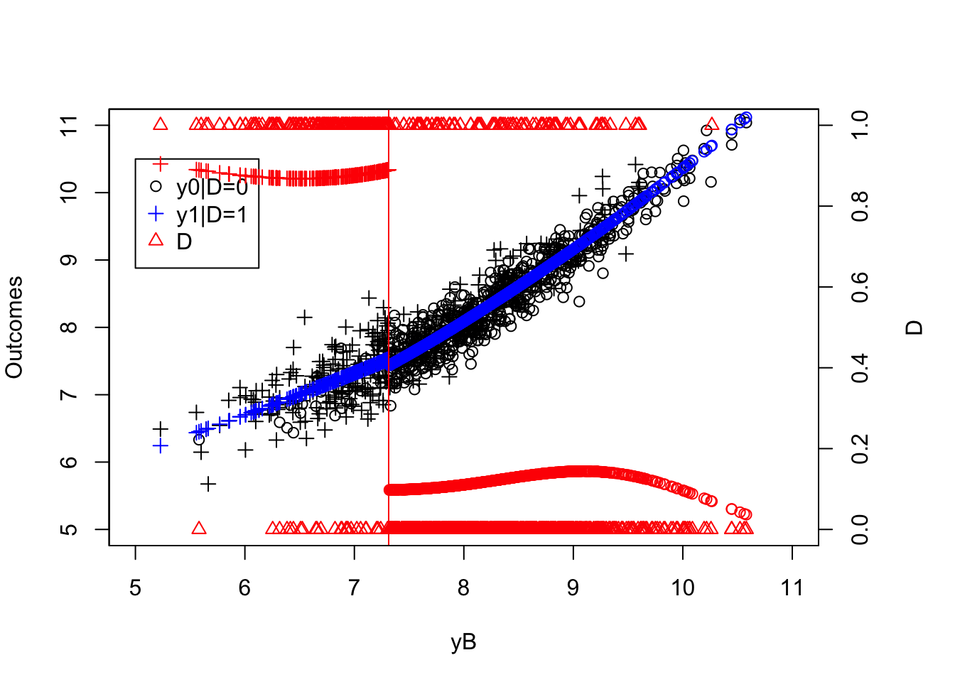
Figure 4.15: Fuzzy RDD estimation with LLR

It is difficult to see the reduced form estimate on Figure 4.15. The numerator of the Wald estimator is equal to 0.1. The Wald estimator of our local average treatment effect is equal to 0.12. The true value of our target parameter (the average treatment effect on the complier at $y_i^B=\bar{y}$) is equal to 0.18, which is the same value as in our example with the Sharp RDD, since the added noise in the participation equation, $V_i$, is independent from potential outcomes, and thus, Assumption 4.10 holds in our example.

Remark. Making $V_i$ correlated with $\eta_i$ or $\mu_i$ in our example would generate a model in which treatment effects are not independent from types (i.e. Assumption 4.10 would not hold). LATE would be different from the treatment on the treated parameter. The formula for the LATE would be: $\Delta^Y_{LATE}(z)=\esp{\alpha_i|yi^B=\bar{y},V_i=0}$. The proof is left as an exercise.

4.2.2.2.2 Estimation using the simplified IV estimator of Imbens and Lemieux

Imbens and Lemieux (2008) propose the following simplified version of the WALD LLR estimator: $\hat{\delta}$ estimated by 2SLS using $\uns{Z_i\leq\bar{z}}$ as an instrument on the sample of observations such as $\bar{z}-h\leq Z_i\leq\bar{z}+h$ is an estimate of $LATE(z)$:

\[\begin{align*} Y_i & = \alpha + \beta (Z_i-\bar{z})\uns{Z_i\leq\bar{z}} + \gamma(Z_i-\bar{z})\uns{Z_i>\bar{z}} + \delta D_i + \epsilon_i \end{align*}\]

It is actually equal to the Wald LLR estimate with uniform kernel and identical bandwidth on each side of the threshold. The bandwidth can be chosen as to be the minimum of the four LLR bandwidths.

Example 4.23 Let’s see how this works in our example.

bw <- min(bwD0,bwD1,bwyS0,bwyS1)
#bw <- 0.4

y.h <- y[log(param['barY'])-bw<yB & yB<log(param['barY'])+bw]
Ds.h <- Ds[log(param['barY'])-bw<yB & yB<log(param['barY'])+bw]
yB.l <- (yB[log(param['barY'])-bw<yB & yB<log(param['barY'])+bw]-log(param['barY']))*S[log(param['barY'])-bw<yB & yB<log(param['barY'])+bw]
yB.r <- (yB[log(param['barY'])-bw<yB & yB<log(param['barY'])+bw]-log(param['barY']))*(1-S[log(param['barY'])-bw<yB & yB<log(param['barY'])+bw])
S.h <- S[log(param['barY'])-bw<yB & yB<log(param['barY'])+bw]

reg.fuzzy.rdd.local.iv <- ivreg(y.h  ~ Ds.h + yB.l + yB.r | S.h + yB.l + yB.r)
delta.rdd.fuzzy.il <- reg.fuzzy.rdd.local.iv$coef[2]
delta.y.tt.rdd.fuzzy <- delta.y.tt.z(param)

With this estimator and using the minimum of the four bandwidths, we estimate the effect of the treatment to be equal to 0.15, while the true effect in the population is equal to 0.18.

Let’s see how this estimator behaves around sampling replications:

monte.carlo.fuzzy.rdd.llr.bw <- function(s,N,param,bw){
  set.seed(s)
  mu <- rnorm(N,param["barmu"],sqrt(param["sigma2mu"]))
  UB <- rnorm(N,0,sqrt(param["sigma2U"]))
  yB <- mu + UB 
  YB <- exp(yB)
  Ds <- rep(0,N)
  V <- rnorm(N,0,sqrt(param["sigma2mu"]+param["sigma2U"]))
  Ds[((yB<=log(param["barY"])) & (V<=param["kappa"])) | ((yB>log(param["barY"])) & (V>param["kappa"])) ] <- 1 
  epsilon <- rnorm(N,0,sqrt(param["sigma2epsilon"]))
  eta<- rnorm(N,0,sqrt(param["sigma2eta"]))
  U0 <- param["rho"]*UB + epsilon
  y0 <- mu +  U0 + param["delta"] + param["gamma"]*(yB-param["baryB"])^2
  alpha <- param["baralpha"]+  param["theta"]*mu + eta
  y1 <- y0+alpha
  Y0 <- exp(y0)
  Y1 <- exp(y1)
  y <- y1*Ds+y0*(1-Ds)
  Y <- Y1*Ds+Y0*(1-Ds)
  Z <- ifelse(yB<=log(param['barY']),1,0)
  y.h <- y[log(param['barY'])-bw<yB & yB<log(param['barY'])+bw]
  Ds.h <- Ds[log(param['barY'])-bw<yB & yB<log(param['barY'])+bw]
  yB.l <- (yB[log(param['barY'])-bw<yB & yB<log(param['barY'])+bw]-log(param['barY']))*Z[log(param['barY'])-bw<yB & yB<log(param['barY'])+bw]
  yB.r <- (yB[log(param['barY'])-bw<yB & yB<log(param['barY'])+bw]-log(param['barY']))*(1-Z[log(param['barY'])-bw<yB & yB<log(param['barY'])+bw])
  Z.h <- Z[log(param['barY'])-bw<yB & yB<log(param['barY'])+bw]
  reg.fuzzy.rdd.local.iv <- ivreg(y.h  ~ Ds.h + yB.l + yB.r | Z.h + yB.l + yB.r)
  delta.rdd.fuzzy.il <- reg.fuzzy.rdd.local.iv$coef[2]
  return(delta.rdd.fuzzy.il)
}

simuls.fuzzy.rdd.llr.bw.N <- function(N,Nsim,param,bw){
  simuls.fuzzy.rdd.llr.bw <- matrix(unlist(lapply(1:Nsim,monte.carlo.fuzzy.rdd.llr.bw,N=N,param=param,bw=bw)),nrow=Nsim,ncol=1,byrow=TRUE)
  colnames(simuls.fuzzy.rdd.llr.bw) <- c('RDD LLR')
  return(simuls.fuzzy.rdd.llr.bw)
}

sf.simuls.fuzzy.rdd.llr.bw.N <- function(N,Nsim,param,bw){
  sfInit(parallel=TRUE,cpus=8)
  sfExport('llr','MSE.llr','param')
  sfLibrary(AER)
  sim <- matrix(unlist(sfLapply(1:Nsim,monte.carlo.fuzzy.rdd.llr.bw,N=N,param=param,bw=bw)),nrow=Nsim,ncol=1,byrow=TRUE)
  sfStop()
  colnames(sim) <- c('RDD LLR')
  return(sim)
}

Nsim <- 1000
#Nsim <- 10
N.sample <- c(100,1000,10000,100000)
#N.sample <- c(100,1000,10000)
#N.sample <- c(100,1000)
#N.sample <- c(100)

simuls.fuzzy.rdd.llr.bw <- lapply(N.sample,sf.simuls.fuzzy.rdd.llr.bw.N,Nsim=Nsim,param=param,bw=bw)
names(simuls.fuzzy.rdd.llr.bw) <- N.sample

Let’s plot the resulting estimates:

par(mfrow=c(2,2))
for (i in 1:length(simuls.fuzzy.rdd.llr.bw)){
  hist(simuls.fuzzy.rdd.llr.bw[[i]][,'RDD LLR'],breaks=30,main=paste('N=',as.character(N.sample[i])),xlab=expression(hat(Delta^yIVRDDLLR)),xlim=c(-0.15,0.55))
  abline(v=delta.y.tt.z(param),col="red")
}

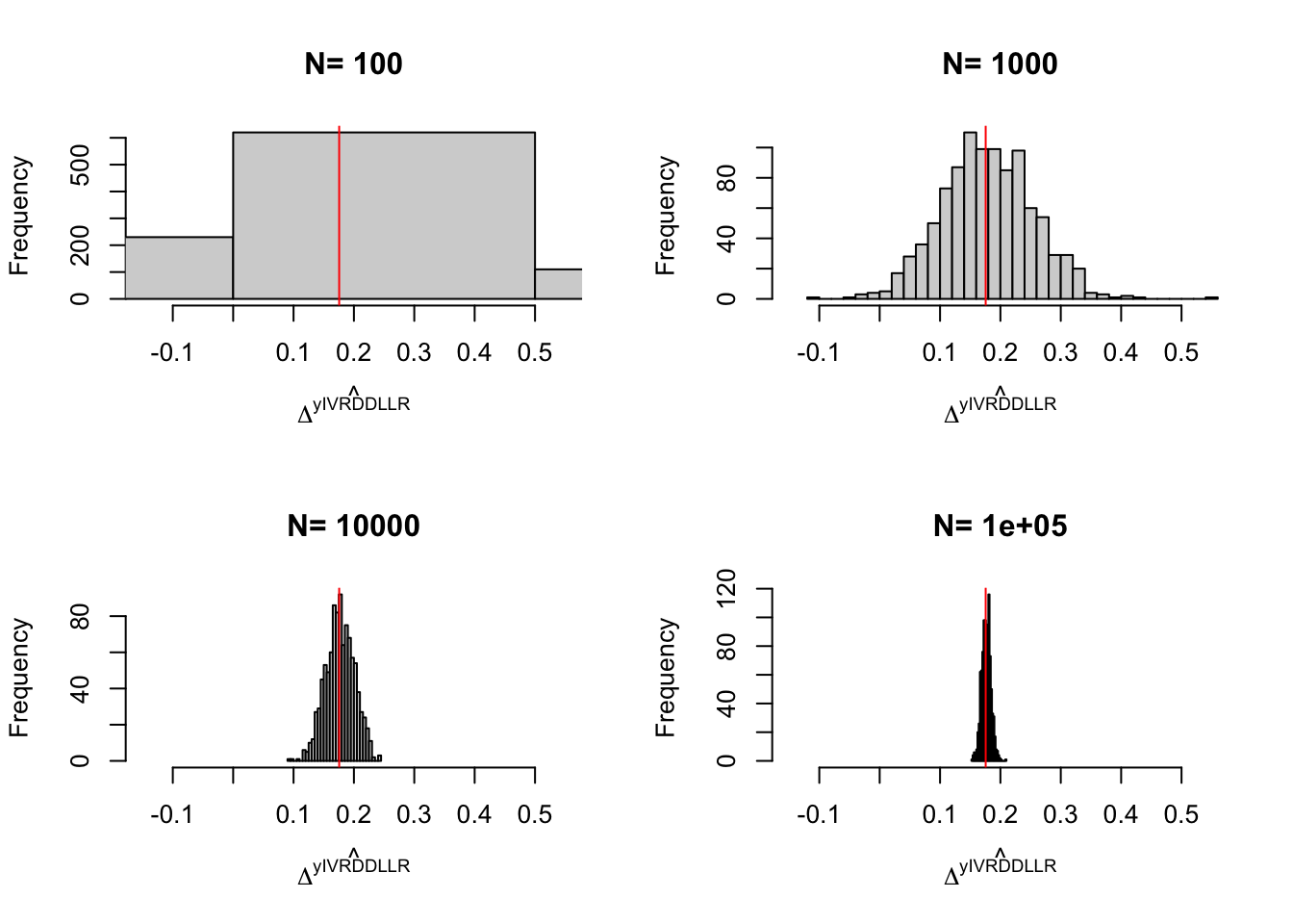
Figure 4.16: Distribution of the $IV RDD LLR$ estimator over replications of samples of different sizes

4.2.2.3 Estimation of sampling noise

We can use several approaches to estimate the sampling noise of the Wald RDDLLR eestimator:

Hahn, Todd and van der Klaauw (2001) derive general CLT results
Imbens and Lemieux (2008) simplify the CLT results and propose a plug-in estimator
Imbens and Lemieux (2008) propose to use the robust variance of the 2SLS estimator
Bootstrap should be valid.

The following theorem derives the CLT-based variance of the simplified Wald RDDLLR estimator:

Theorem 4.8 (Asymptotic Variance of the LLR-IV Estimator) The variance of the simplified LLR-IV Estimator in a Fuzzy Design can be approximated by:

\[\begin{align*} \var{\hat{\Delta}_{LLRRDDIV}} & \approx \frac{1}{Nh}\left(\frac{1}{\tau^2_{D}}V_{\tau_Y}+\frac{\tau^2_{Y}}{\tau^4_{D}}V_{\tau_D}-2\frac{\tau_{Y}}{\tau^3_{D}}C_{\tau_Y,\tau_D}\right), \end{align*}\]

with

\[\begin{align*} \tau_{D} & = \lim_{e\rightarrow 0^{+}}\esp{D_i|Z_i=\bar{z}+e}-\lim_{e\rightarrow 0^{+}}\esp{D_i|Z_i=\bar{z}-e}\\ V_{\tau_Y} & = \frac{4}{f_Z(\bar{z})}\left(\sigma^2_{Y^r}+\sigma^2_{Y^l}\right) \qquad V_{\tau_D} = \frac{4}{f_Z(\bar{z})}\left(\sigma^2_{D^r}+\sigma^2_{D^l}\right)\\ C_{\tau_Y,\tau_D}& = \frac{4}{f_Z(\bar{z})}\left(C_{YD^r}+C_{YD^l}\right) \qquad \sigma^2_{Y^r} = \lim_{e\rightarrow 0^{+}}\var{Y_i|Z_i=\bar{z}+e} \\ C_{YD^r} & = \lim_{e\rightarrow 0^{+}}\cov{Y_i,D_i|Z_i=\bar{z}+e} \end{align*}\]

Proof. Hahn, Todd and van der Klaauw (2001) and Imbens and Lemieux (2008).

Another way is tu simply use the robust standard errors from the 2SLS estimator.

Example 4.24 Let’s see what happens with this estimator of sampling noise in our example.

The estimated 99% sampling noise the robust standard errors from the 2SLS estimator is 0.37. The true 99% sampling noise of Wald RDDLLR estimated by Monte Carlo simulations is 0.39.

4.3 Difference In Differences

In Difference In Differences (a.k.a. DID), the difference between treated and untreated before the treatment is used to approximate selection bias. As a consequence, DID works by correcting the With/Without comparison after treatment by the With/Without comparison before treatment and hopes that it is enough to recover the TT. Hence the name Difference in Differences (DID), since the estimator, in its simplest form, is a difference between two differences. In this section, we are going to look at identification using DID, estimation and estimation of sampling noise. At first, we are going to assume that we have only access to two time periods. In that case, estimation and inference are pretty straightforward. We will then examine the case of several time periods, but we will first allow for only one treatment date. In that case, we will introduce the standard tools used by applied researchers to analyze these types of designs: the event study graph and the Two-Way Fixed Effects estimator (a.k.a. TWFE). We will determine which effect is estimated by the TWFE estimator and what are the goals of the event study graph. We will then look at the most complex case: the staggered design, where we have several time periods (strictly more than two) and the date of treatment differs across units. In the staggered design, troubles start appearing for the TWFE estimator. We will survey these problems and the proposed solutions to address them. Finally, we will look at the combination of DID with instrumental variables (the DID-IV estimator) and see which specific types of problems happen there as well. Let’s get to it.

4.3.1 Difference In Differences with two time periods

Before getting into the rigorous derivations, let’s start with a very simple illustration using our workhorse example.

Example 4.25 How does DID perform and what does it look like in our example model?

Let’s first generate a dataset with selection bias.

\[\begin{align*} y_i^1 & = y_i^0+\bar{\alpha}+\theta\mu_i+\eta_i \\ y_i^0 & = \mu_i+\delta+U_i^0 \\ U_i^0 & = \rho U_i^B+\epsilon_i \\ y_i^B & =\mu_i+U_i^B \\ U_i^B & \sim\mathcal{N}(0,\sigma^2_{U}) \\ \mu_i & \sim\mathcal{N}(\bar{\mu},\sigma^2_{\mu}) \\ D_i & = \uns{y_i^B+ V_i\leq\bar{y}} \\ V_i & = \gamma(\mu_i-\bar{\mu}) + \omega_i \\ (\eta_i,\omega_i) & \sim\mathcal{N}(0,0,\sigma^2_{\eta},\sigma^2_{\omega},\rho_{\eta,\omega}) \end{align*}\]

param <- c(8,.5,.28,1500,0.9,0.01,0.05,0.05,0.05,0.1,0.1,7.98,0.28,0)
names(param) <- c("barmu","sigma2mu","sigma2U","barY","rho","theta","sigma2epsilon","sigma2eta","delta","baralpha","gamma","baryB","sigma2omega","rhoetaomega")

set.seed(1234)
N <-1000
cov.eta.omega <- matrix(c(param["sigma2eta"],param["rhoetaomega"]*sqrt(param["sigma2eta"]*param["sigma2omega"]),param["rhoetaomega"]*sqrt(param["sigma2eta"]*param["sigma2omega"]),param["sigma2omega"]),ncol=2,nrow=2)
eta.omega <- as.data.frame(mvrnorm(N,c(0,0),cov.eta.omega))
colnames(eta.omega) <- c('eta','omega')
mu <- rnorm(N,param["barmu"],sqrt(param["sigma2mu"]))
UB <- rnorm(N,0,sqrt(param["sigma2U"]))
yB <- mu + UB 
YB <- exp(yB)
Ds <- rep(0,N)
V <- param["gamma"]*(mu-param["barmu"])+eta.omega$omega
Ds[yB+V<=log(param["barY"])] <- 1 
epsilon <- rnorm(N,0,sqrt(param["sigma2epsilon"]))
U0 <- param["rho"]*UB + epsilon
y0 <- mu +  U0 + param["delta"]
alpha <- param["baralpha"]+  param["theta"]*mu + eta.omega$eta
y1 <- y0+alpha
Y0 <- exp(y0)
Y1 <- exp(y1)
y <- y1*Ds+y0*(1-Ds)
Y <- Y1*Ds+Y0*(1-Ds)

Let’s see how DID works on this data.

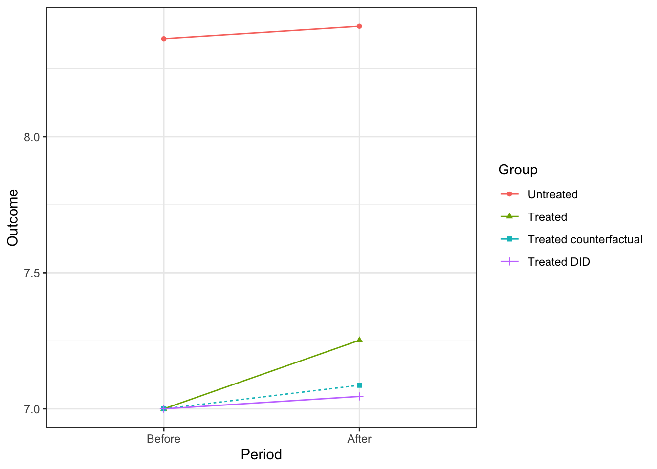
Figure 4.17: Evolution of average outcomes in the treated and control group

Figure 4.17 shows the evolution of the mean log-outcomes for the treated and untreated groups over time in our simulated dataset. We can see that in the Before period, outcomes ($y_i^B$ in that case) are much higher for the non participants than for the participants, in agreement with the selection rule that makes participation into the program more likely for individuals with lower pre-treatment outcomes. The With/Without difference in outcomes before the program takes place is $\hat{\Delta}^{y^B}_{WW}=$ -1.361. Second, we see that the difference between participants and non-participants decreases after receiving the treatment. This is because the outcomes of the participants increase faster than the outcomes of the non participants. As a consequence, the With/Without difference in outcomes after the program takes place is $\hat{\Delta}^{y}_{WW}=$ -1.154. The DID estimator is built by comparing these two differences. In our example, $\hat{\Delta}^{y}_{DID}=$ 0.206. It is not too far from the true treatment effect of $\hat{\Delta}^{y}_{TT}=$ 0.165.

Figure 4.17 also demonstrates that the DID estimator can also be seen as the difference between the Before/After differences in outcomes of the treated and the untreated. The Before/After difference in outcomes for the non participants is $\hat{\Delta}^{y}_{BA|D=0}=$ 0.046 while the Before/After difference for the participants is $\hat{\Delta}^{y}_{BA|D=1}=$ 0.252, leading to the same DID estimand. One way to understand the DID estimator is to see it as recreating the counterfactual trajectory of the participants (show as a discontinuous line on Figure 4.17) by using the trajectory of the non participants and making it start at the pre-treatment level of the participants. This estimated counterfactual trajectory is shown as the purple continuous line at the bottom of Figure 4.17. In our example, the true counterfactual trajectory (the discontinuous line) and the estimated counterfactual trajectory almost coincide, making the estimated counterfactual outcome of the participants very close to their true counterfactual outcome (7.046 vs 7.087). The difference between these two quantities measures the bias of the DID estimator, and we can see that it is very low in our example. The fact that the Before/After difference in outcomes for the non participants approximates well the counterfactual Before/After difference in outcomes for the participants is THE crucial assumption of the DID estimator. It is called the parallel trends assumption.

4.3.1.1 Identification

The formal setting for introducing the DID estimator is to start with two time periods, Before and After ($t=B$ and $t=A$ respectively). Outcomes with and without the treatment in both periods are denoted $Y^d_{i,t}$, for $d\in\left\{0,1\right\}$ and $t\in\left\{B,A\right\}$. Treatment participation in both periods is denoted $D_{i,t}$ for $t\in\left\{B,A\right\}$. In the Before period, the treatment is unavailable, so that we get to observe the potential outcomes of the agents in the absence of the treatment. These two very specific requirements of DID are encoded in the following way:

Hypothesis 4.12 (No Treatment in the Before Period) We assume that no unit in the population receives the treatment in the Before period: $D_{i,B}=0$, $\forall i$ and not all units receive the program in the After period, but some units receive it: $0<\Pr(D_{i,A}=1)<1$.

Under Assumption 4.12, and without loss of generality, we are going to write $D_i=D_{i,A}$.

Hypothesis 4.13 (No Anticipation Effects) We assume that, in the Before period, agents cannot anticipate that the program will happen in the After period, or that they do not change their behavior as a consequence: $Y_{i,B}=Y^0_{i,B}$, $\forall i$.

A consequence of Assumptions 4.12 and 4.13 is that we can write observed outcomes as a function of treatment and potential outcomes using the usual switching equation:

\[\begin{align}\label{eqn:switchDID} Y_{i,t} & = Y^1_{i,t}D_{i,t} + Y^0_{i,t}(1-D_{i,t}). \end{align}\]

The final very important assumption that we can make is to assume that the trends in the potential outcomes in the absence the treatment are the same for the treated and the untreated units:

Hypothesis 4.14 (Parallel Trends) We assume that the trends in the potential outcomes in the absence the treatment are the same for the treated and the untreated units:

\[\begin{align*} \esp{Y^0_{i,A}|D_i=1} - \esp{Y^0_{i,B}|D_i=1} & = \esp{Y^0_{i,A}|D_i=0} - \esp{Y^0_{i,B}|D_i=0}. \end{align*}\]

Assumption 4.14 is actually equivalent to assuming that selection bias is constant over time. This is what this very simple lemma shows:

Lemma 4.3 (Parallel Trends is Constant Selection Bias) Assumption 4.14 is equivalent to assuming that selection bias is constant over time:

\[\begin{align*} \esp{Y^0_{i,A}|D_i=1} - \esp{Y^0_{i,A}|D_i=0} & = \esp{Y^0_{i,B}|D_i=1} - \esp{Y^0_{i,B}|D_i=0} . \end{align*}\]

Proof. The proof follows immediately by adding $\esp{Y^0_{i,B}|D_i=1}-\esp{Y^0_{i,A}|D_i=0}$ to both sides of the equation in Assumption 4.14.

Under these assumptions, we are ready to state the main identification result of this section:

Theorem 4.9 (DID identifies TT) Under Assumptions 4.12, 4.13 and 4.14, the DID estimator identifies the average effect of the Treatment on the Treated after the treatment:

\[\begin{align*} \Delta_{DID}^{Y} & = \Delta^{Y_A}_{TT}, \end{align*}\]

with:

\[\begin{align*} \Delta^Y_{DID} & = \esp{Y_{i,A}|D_i=1} - \esp{Y_{i,B}|D_i=1} - (\esp{Y_{i,A}|D_i=0} - \esp{Y_{i,B}|D_i=0}),\\ \Delta^{Y_A}_{TT} & = \esp{Y^1_{i,A}-Y^0_{i,A}|D_{i}=1}. \end{align*}\]

Proof. \[\begin{align*} \Delta^Y_{DID} & = \esp{Y_{i,A}|D_i=1}-\esp{Y_{i,B}|D_i=1}-(\esp{Y_{i,A}|D_i=0}-\esp{Y_{i,B}|D_i=0}) \\ & = \esp{Y^1_{i,A}|D_i=1}-\esp{Y^0_{i,B}|D_i=1}-(\esp{Y^0_{i,A}|D_i=0}-\esp{Y^0_{i,B}|D_i=0})\\ & = \esp{Y^1_{i,A}|D_i=1}-\left(\esp{Y^0_{i,A}|D_i=0}+(\esp{Y^0_{i,B}|D_i=1}-\esp{Y^0_{i,B}|D_i=0})\right) \end{align*}\]

where the second equality follows from Assumptions 4.12 and 4.13 and the switching equation, and the third equality follows from Lemma 4.3. Under Assumption 4.14, we have:

\[\begin{align*} \esp{Y^0_{i,A}|D_i=1} & = \esp{Y^0_{i,A}|D_i=0} + (\esp{Y^0_{i,B}|D_i=1}-\esp{Y^0_{i,B}|D_i=0}) \end{align*}\]

As a consequence, we have:

\[\begin{align*} \Delta^Y_{DID} & = \esp{Y^1_{i,A}|D_i=1}-\esp{Y^0_{i,A}|D_i=1}\\ & = \esp{Y^1_{i,A}-Y^0_{i,A}|D_i=1}\\ & = \Delta^{Y_A}_{TT}. \end{align*}\]

Example 4.26 How does the DID estimator behave in our example?

The Before/After comparison among the participants is equal to $\hat{\Delta}^{y}_{BA|D=1}=$ 0.252. The Before/After comparison among the non-participants is equal to $\hat{\Delta}^{y}_{BA|D=0}=$ 0.046. The DID estimator is thus equal to $\hat{\Delta}^{y}_{DID}=\hat{\Delta}^{y}_{BA|D=1}-\hat{\Delta}^{y}_{BA|D=0}=$ 0.252 $-$ 0.046 $=$ 0.206. It is also equal to the difference between the before and after With/Without estimators. The Before With/Without estimator is equal to $\hat{\Delta}^{y^B}_{WW}=$ -1.361. The After With/Without estimator is equal to $\hat{\Delta}^{y}_{WW}=$ -1.154. The DID estimator is thus equal to $\hat{\Delta}^{y}_{DID}=\hat{\Delta}^{y}_{WW}-\hat{\Delta}^{y^B}_{WW}=$ -1.154 $-($ -1.361 $)=$ 0.206. This is not too far from the true effect of the treatment in the sample which is equal to $\hat{\Delta}^{y}_{TT}=$ 0.165.

Now, another very important question is whether the DID estimator is consistent, that is whether it is equal to $\Delta^{y}_{TT}$ in our model. A necessary and sufficient condition for that is for the Parallel Trends Assumption 4.14 to hold. Indeed, it can be shown that the bias of the DID estimator is $\Delta^{y}_{B(DID)}=\Delta^{y}_{DID}-\Delta^{y}_{TT}=$ $\esp{y^0_{i}|D_i=1} - \esp{y^B_{i}|D_i=1}-(\esp{y^0_{i}|D_i=0} - \esp{y^B_{i}|D_i=0})$. Let us derive $\Delta^{y}_{B(DID)}$ in our example. Let us compute the trend in potential outcomes among the treated:

\[\begin{align*} \esp{y^0_{i,A}|D_i=1} & - \esp{y^0_{i,B}|D_i=1} \\ & = \esp{y^0_{i}|D_i=1} - \esp{y^B_{i}|D_i=1} \\ & = \esp{\mu_i+\delta+U_i^0|D_i=1}-\esp{\mu_i+U_i^B|D_i=1} \\ & = \esp{\mu_i|D_i=1}+\delta+\esp{U_i^0|D_i=1}\\ & \phantom{=}-\esp{\mu_i|D_i=1}-\esp{U_i^B|D_i=1} \\ & = \delta + \esp{\rho U_i^B+\epsilon_i|D_i=1}-\esp{U_i^B|D_i=1}\\ & = \delta -(1-\rho)\esp{U_i^B|D_i=1}. \end{align*}\]

Following the same line of reasoning, the trend in potential outcomes among the untreated is:

\[\begin{align*} \esp{y^0_{i}|D_i=0} - \esp{y^B_{i}|D_i=0} & = \delta -(1-\rho)\esp{U_i^B|D_i=0}. \end{align*}\]

As a consequence, the bias of the DID estimator in our model is:

\[\begin{align*} \Delta^{y}_{B(DID)} & = -(1-\rho)(\esp{U_i^B|D_i=1}-\esp{U_i^B|D_i=0}) \\ & = -(1-\rho)(\esp{U_i^B|\mu_i+U_i^B+V_i\leq\bar{y}}-\esp{U_i^B|\mu_i+U_i^B+V_i>\bar{y}}) \end{align*}\]

Is this zero? The answer actually is that it is not. In order to see why, notice intuitively that the conditional expectation of $U_i^B$ is taken conditional on something correlated with $U_i^B$ being above or below some threshold. As a consequence, the two values whose difference is taken in the parenthesis cannot be equal. More formally, let us derive the formula for the bias of the DID estimator in our model, using the formula for the expectation of a truncated bivariate normal distribution:

\[\begin{align*} \Delta^{y}_{B(DID)} & = -(1-\rho)(\esp{U_i^B|\mu_i+U_i^B+V_i\leq\bar{y}}-\esp{U_i^B|\mu_i+U_i^B+V_i>\bar{y}}) \\ & = (1-\rho)\left(\frac{\sigma^2_U}{(1+\gamma^2)\sigma^2_{\mu}+\sigma^2_U+\sigma^2_{\omega}}\right) \left(\frac{\phi\left(\frac{\bar{y}-\bar{\mu}}{(1+\gamma^2)\sigma^2_{\mu}+\sigma^2_U+\sigma^2_{\omega}}\right)} {\Phi\left(\frac{\bar{y}-\bar{\mu}}{(1+\gamma^2)\sigma^2_{\mu}+\sigma^2_U+\sigma^2_{\omega}}\right)} +\frac{\phi\left(\frac{\bar{y}-\bar{\mu}}{(1+\gamma^2)\sigma^2_{\mu}+\sigma^2_U+\sigma^2_{\omega}}\right)} {1-\Phi\left(\frac{\bar{y}-\bar{\mu}}{(1+\gamma^2)\sigma^2_{\mu}+\sigma^2_U+\sigma^2_{\omega}}\right)} \right) \end{align*}\]

In order to compute the value of this parameter, and of the average treatment effect, we are going to use the package tmtvnorm which provides the moments from a truncated multivariate normal variable. Here, we use the distribution of $(\alpha_i,U_i^B,\mu_i+U_i^B+V_i)$ which is normal with mean $(\bar{\alpha}+\theta\bar{\mu},0,\bar{\mu})$ and covariance matrix $\mathbf{D}$ with:

\[\begin{align*} \mathbf{D} &= \left(\begin{array}{ccc} \theta^2\sigma^2_{\mu}+ \sigma^2_{\eta} & 0 & (\theta+\gamma\theta)\sigma^2_{\mu}+\rho_{\eta,\omega}\sigma_{\eta}\sigma_{\omega}\\ 0 & \sigma^2_U & \sigma^2_U \\ (\theta+\gamma\theta)\sigma^2_{\mu}+\rho_{\eta,\omega}\sigma_{\eta}\sigma_{\omega}& \sigma^2_U & (1+\gamma^2)\sigma^2_{\mu}+\sigma^2_U+\sigma^2_{\omega} \end{array}\right) \end{align*}\]

mean.alpha.UB.yBV <- c(param['baralpha']+param['barmu']*param['theta'],0,param['barmu'])
cov.alpha.UB.yBV <- matrix(c(param['theta']^2*param['sigma2mu']+param['sigma2eta'],
                             0,
                             (param['theta']+param['gamma']*param['theta'])*param['sigma2mu']+param['rhoetaomega']*param['sigma2eta']*param['sigma2omega'],
                             0, 
                             param['sigma2U'],
                             param['sigma2U'],
                             (param['theta']+param['gamma']*param['theta'])*param['sigma2mu']+param['rhoetaomega']*param['sigma2eta']*param['sigma2omega'],
                             param['sigma2U'],
                            (1+param['gamma']^2)*param['sigma2mu']+param['sigma2U']+param['sigma2omega']),3,3,byrow=TRUE)

# cuts
#non participants
lower.cut.D0 <- c(-Inf,-Inf,log(param['barY']))
upper.cut.D0 <- c(Inf,Inf,Inf)
# participants
lower.cut.D1 <- c(-Inf,-Inf,-Inf)
upper.cut.D1 <- c(Inf,Inf,log(param['barY']))

# means 
TT.pop <- mtmvnorm(mean=mean.alpha.UB.yBV,sigma=cov.alpha.UB.yBV,lower=lower.cut.D1,upper=upper.cut.D1,doComputeVariance=FALSE)[[1]][[1]]
mean.UB.D0 <- mtmvnorm(mean=mean.alpha.UB.yBV,sigma=cov.alpha.UB.yBV,lower=lower.cut.D0,upper=upper.cut.D0,doComputeVariance=FALSE)[[1]][[2]]
mean.UB.D1 <- mtmvnorm(mean=mean.alpha.UB.yBV,sigma=cov.alpha.UB.yBV,lower=lower.cut.D1,upper=upper.cut.D1,doComputeVariance=FALSE)[[1]][[2]]
B.DID <- -(1-param['rho'])*(mean.UB.D1-mean.UB.D0)

In our example, the population $TT$ is equal to $\Delta^y_{TT}=$ 0.173. The DID estimator is equal to $\Delta^y_{DID}=$ 0.211. As a consequence, the bias of the DID estimator is equal to $\Delta^y_{B(DID)}=$ 0.046.

In order to make the DID estimator consistent for the $TT$ parameter, we need to impose that $\rho=1$. When shocks are permanent, their bias remains constant over time and thus DID can estimate it without error. Let us generate new data that are compatible with that assumption.

set.seed(1234)
N <-1000
param["rho"] <- 1
cov.eta.omega <- matrix(c(param["sigma2eta"],param["rhoetaomega"]*sqrt(param["sigma2eta"]*param["sigma2omega"]),param["rhoetaomega"]*sqrt(param["sigma2eta"]*param["sigma2omega"]),param["sigma2omega"]),ncol=2,nrow=2)
eta.omega <- as.data.frame(mvrnorm(N,c(0,0),cov.eta.omega))
colnames(eta.omega) <- c('eta','omega')
mu <- rnorm(N,param["barmu"],sqrt(param["sigma2mu"]))
UB <- rnorm(N,0,sqrt(param["sigma2U"]))
yB <- mu + UB 
YB <- exp(yB)
Ds <- rep(0,N)
V <- param["gamma"]*(mu-param["barmu"])+eta.omega$omega
Ds[yB+V<=log(param["barY"])] <- 1 
epsilon <- rnorm(N,0,sqrt(param["sigma2epsilon"]))
U0 <- param["rho"]*UB + epsilon
y0 <- mu +  U0 + param["delta"]
alpha <- param["baralpha"]+  param["theta"]*mu + eta.omega$eta
y1 <- y0+alpha
Y0 <- exp(y0)
Y1 <- exp(y1)
y <- y1*Ds+y0*(1-Ds)
Y <- Y1*Ds+Y0*(1-Ds)

Let’s see how DID works on this data.

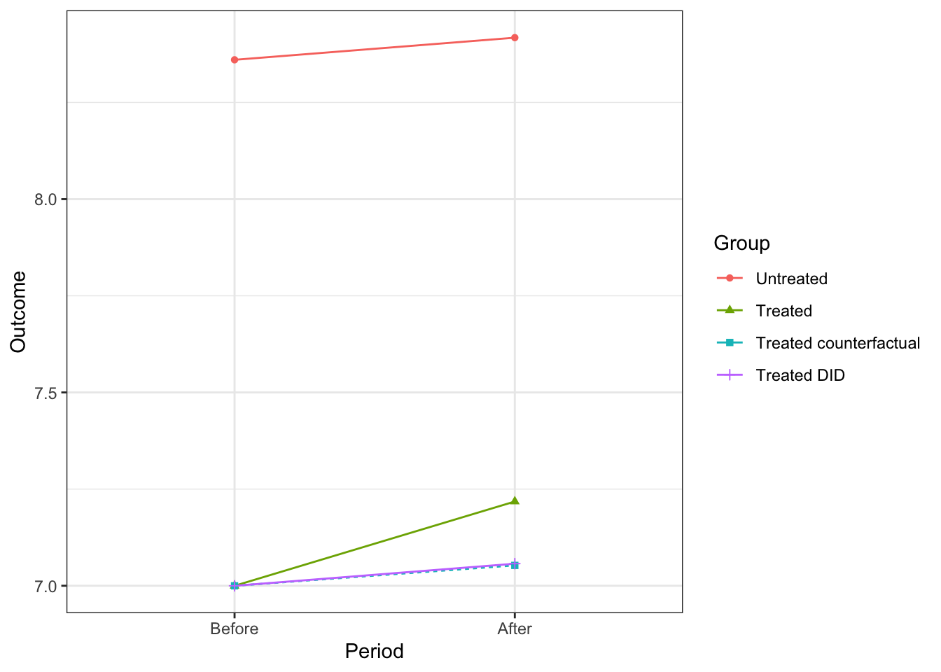
Figure 4.18: Evolution of average outcomes in the treated and control group when the Parallel Trends Assumption holds

Now, the counterfactual change in outcome for the treated and its approximation using the trend experienced by the untreated are extremely close, as the curves Treated counterfactual and Treated DID show on Figure 4.18.

4.3.1.2 Estimation

Estimation of $TT$ under the $DID$ assumptions can be performed in a variety of ways: using directly the DID formula, using OLS with group fixed effects, using OLS with individual and time dummy variables, using first differences and using the within transformation (also known as the Two-Way Fixed Effects or TWFE estimator). With only two periods of data and a fully balanced panel, all of these estimators are actually numerically equivalent. Let’s examine them in turn.

4.3.1.2.1 Using the DID formula

One could go directly and use the DID formula of Theorem 4.9. The sample DID estimator is thus equal to:

\[\begin{align*} \hat{\Delta}^Y_{DID} & = \frac{\sum_{i=1}^NY_{i,A}D_i}{\sum_{i=1}^ND_i} -\frac{\sum_{i=1}^NY_{i,B}D_i}{\sum_{i=1}^ND_i} - \left(\frac{\sum_{i=1}^NY_{i,A}(1-D_i)}{\sum_{i=1}^N(1-D_i)} -\frac{\sum_{i=1}^NY_{i,B}(1-D_i)}{\sum_{i=1}^N(1-D_i)}\right). \end{align*}\]

Example 4.27 In our example, let’s see how this estimator works.

The Before/After comparison among the participants is equal to $\hat{\Delta}^{y}_{BA|D=1}=$ 0.218. The Before/After comparison among the non-participants is equal to $\hat{\Delta}^{y}_{BA|D=0}=$ 0.057. The DID estimator is thus equal to $\hat{\Delta}^{y}_{DID}=\hat{\Delta}^{y}_{BA|D=1}-\hat{\Delta}^{y}_{BA|D=0}=$ 0.218 $-$ 0.057 $=$ 0.161. It is also equal to the difference between the before and after With/Without estimators. The Before With/Without estimator is equal to $\hat{\Delta}^{y^B}_{WW}=$ -1.361. The After With/Without estimator is equal to $\hat{\Delta}^{y}_{WW}=$ -1.2. The DID estimator is thus equal to $\hat{\Delta}^{y}_{DID}=\hat{\Delta}^{y}_{WW}-\hat{\Delta}^{y^B}_{WW}=$ -1.2 $-($ -1.361 $)=$ 0.161. This is not too far from the true effect of the treatment in the sample which is equal to $\hat{\Delta}^{y}_{TT}=$ 0.165. In the population, the $TT$ parameter has not changed, since its computation does not involve $\rho$. We still have $\Delta^y_{TT}=$ 0.173.

4.3.1.2.2 Using the Least Squares pooling DID estimator

The most basic regression-based way to implement DID is to run a linear regression of outcomes on a treatment group dummy, a time dummy and their interaction. The interaction captures the effect of the treatment estimated using DID. The way it works is as follows: estimate the following equation using OLS and use $\hat{\beta}_{OLS}$ as your DID estimate: $\hat{\beta}_{OLS}=\hat{\Delta}^{Y}_{DID}$. \[\begin{align*} Y_i & = \alpha + \mu D_i + \delta T_i + \beta D_iT_i + \epsilon_i. \end{align*}\] $D_i$ is our usual treatment indicator while $T_i$ takes value one when observation $i$ is observed in the After and zero otherwise.

Example 4.28 Let’s see how this works in our example.

Before estimating the model, we need to build a data frame with all the necessary variables.

# building a data frame
data.DID <- as.data.frame(cbind(c(y,yB),c(Ds,Ds),c(rep(1,N),rep(0,N))))
colnames(data.DID) <- c('y','D','T')

# running the OLS regression
reg.DID <- lm(y ~ D + T + D*T,data = data.DID)

# coefficients
yB.D0.reg <-  coef(reg.DID)[[1]]
WW.before.reg <-  coef(reg.DID)[[2]]
BA.untreated.reg <- coef(reg.DID)[[3]]
DID.est.reg <- coef(reg.DID)[[4]]

# comparisons
yB.D0.sample <- mean(yB[Ds==0])

The estimate of $\hat{\beta}_{OLS}$ in our sample is equal to 0.161. It is exactly equal to $\hat{\Delta}^{y}_{DID}$ as estimated just above. What is interesting with the regression-based DID approach is that the other coefficients in the regression have a direct interpretation. For example, the constant $\alpha$ estimates the mean outcome in the untreated group before the treatment. In our case, we have $\hat{\alpha}_OLS=$ 8.36. Remember that in our sample, the average outcomes of the untreated before the treatment is equal to $\hatesp{y_i^B|D_i=0}=$ 8.36. $\mu$, the coefficient in front of the $D_i$ dummy, estimates the With/Without estimator before the treatment. In our case, we have $\hat{\mu}_{OLS}=$ -1.361. Remember that in our sample, the With/Without estimator before the treatment is equal to $\hat{\Delta}^{y^B}_{WW}=$ -1.361. $\delta$, the coefficient in front of the $T_i$ dummy, estimates the Before/After change in outcomes among the untreated. In our case, we have $\hat{\delta}_{OLS}=$ 0.057. Remember that in our sample, the Before/After estimator among the untreated is equal to $\hat{\Delta}^{y}_{BA|D=0}=$ 0.057.

Remark. A pretty cool property of the regression-based DID estimator is that is does not require panel data. It works even with repeated cross sections, i.e. when observations are drawn from the same population in both periods but are not the same.

4.3.1.2.3 Using First Differences

In the presence of panel data, an alternative to the regression-based DID estimator is the first-difference estimator. It simply regresses the change over time in outcomes on the treatment dummy: \[\begin{align*} Y_{i,A}-Y_{i,B} & = \alpha^{FD} + \beta^{FD} D_i + \epsilon^{FD}_i. \end{align*}\] The coefficient $\beta^{FD}$ estimated by OLS is an estimate of the DID parameter.

Example 4.29 Let’s see how this works in our example.

Before running the model, we need to generate first the differenced estimates. One very simple way to do that is simply to take the difference between the before and the after outcome vectors.

# building a data frame
data.FD <- as.data.frame(cbind(y-yB,Ds))
colnames(data.FD) <- c('BAy','D')

# running the OLS regression
reg.FD <- lm(BAy ~ D,data = data.FD)

# coefficients
BA.untreated.FD <- coef(reg.FD)[[1]]
DID.est.FD <- coef(reg.FD)[[2]]

The estimate of $\hat{\beta}^{FD}_{OLS}$ in our sample is equal to 0.161. It is exactly equal to $\hat{\Delta}^{y}_{DID}$ as estimated just above. Note also that $\alpha^{FD}$ estimates the Before/After change in outcomes among the untreated. In our case, we have $\hat{\alpha}^{FD}_{OLS}=$ 0.057. Remember that in our sample, the Before/After estimator among the untreated is equal to $\hat{\Delta}^{y}_{BA|D=0}=$ 0.057.

4.3.1.2.4 Using the Least Squares Dummy Variables estimator

One very computer-intensive way to estimate $TT$ in a DID setting is to use the OLS estimator supplemented with dummies for each observation and for each time period, also called the Least-Squares Dummy Variables estimator. In practice, the estimator is based on the following regression: \[\begin{align*} Y_{i,t} & = \sum_{j=1}^N\mu_j\uns{j=i} + \sum_{l=0}^1\delta_l\uns{l=t} + \beta^{LSDV} D_{i,t} + \epsilon^{LSDV}_{i,t}. \end{align*}\] The notation is generally simplified as follows: \[\begin{align*} Y_{i,t} & = \mu_i + \delta_t + \beta^{TWFE} D_{i,t} + \epsilon^{TWFE}_{i,t}, \end{align*}\]

This last estimator is generally called the Two-Way Fixed Effects estimator, since it has two-sets of so-called fixed effects (individual fixed effects, $\mu_i$, and time fixed effects $\delta_t$). I will write it using this second, more compact, formulation, but I think the first formulation encapsulates better how the Least-Squares Dummy Variables estimator works. In what follows, we will see other ways of estimating the Two-Way Fixed Effects model, but for now, let us focus on the Least-Squares Dummy Variables estimator. The way it works is simply by throwing a bunch of dummy variables in the regression.

Example 4.30 Let’s see how the Least Squares Dummy Variable works in our example. For that, we need to generate one dummy variable for each individual $i$ in our sample. This is made simple by the factor function in R. We are also going to run the model without a constant, so that all the fixed effects are identified.

# adding one column to the DID data frame with the individual index for each observation of the same $i$
data.DID$indiv <- as.factor(c(1:N,1:N))
# generating Dit (time varying)
data.DID$Dit <- data.DID$D*data.DID$T
# running the LSDV estimator
reg.LSDV <- lm(y~-1 + Dit + as.factor(T) + indiv,data=data.DID)
# result
DID.est.LSDV <- coef(reg.LSDV)[[1]]

The Least-Squares Dummy Variables estimate of $TT$ is equal to: $\hat{\beta}^{LSDV}=$ 0.161.

Remark. The term fixed effect is specific to the panel data literature in econometrics. It refers to the fact that both $\mu_i$ and $\delta_t$ are allowed to be correlated with $D_{i,t}$ in this model. This is in contrast to the random effects model where $\mu_i$ and $\delta_t$ are assumed to be independent of the regressors of interest.

4.3.1.2.5 Using the Within estimator

You might have noticed that the Least-Squares Dummy Variables estimator took some time to compute on your computer. This is because it requires the inversion of a very large matrix, as large as the number of fixed effects plus one. The size of this computation increases as the number of observation and time periods increases, meaning that this computation might become practically unfeasible in very large datasets. Several tricks have been developed to decrease the computational burden of the estimation of the Two-Way Fixed Effects model. One approach is to use the First Difference estimator. Another approach is the Within estimator. The way the Within estimator works is by taking the difference between each observation and its mean over time or over individuals. More precisely, the Within estimator estimates the following model by OLS: \[\begin{align*} Y_{i,t}-\frac{1}{2}\sum_{t=0}^1Y_{i,t} & = \delta^{W}_t + \beta^{W}(D_{i,t}-\frac{1}{2}\sum_{t=0}^1D_{i,t}) + \epsilon^{W}_{i,t}. \end{align*}\]

The reason why this trick works is because of the shape of the Two-Way Fixed Effects model. Indeed, taking the average of the Two-Way Fixed Effects model over time gives: \[\begin{align*} \frac{1}{2}\sum_{t=0}^1Y_{i,t} & = \mu_i + \frac{1}{2}\sum_{t=0}^1\delta_t + \beta^{TWFE}\frac{1}{2}\sum_{t=0}^1D_{i,t} + \frac{1}{2}\sum_{t=0}^1\epsilon^{TWFE}_{i,t}. \end{align*}\] Taking the difference between the Two-Way Fixed Effects model and its time-averaged version gives the Within estimator. The key is that the differencing gets rid of the individual fixed effects parameter $\mu_i$ and thus makes it unnecessary to estimate it. The set of parameters to estimate is thus much smaller than in the Least-Squares Dummy Variables estimator.

Example 4.31 Let’s see how the Within estimator works in our example. For that, we need to compute the average over time of the outcome and of the treatment for each observation in our dataset. This is made simple by the summarize function of the dplyr package.

# generating the time means of Y and Dit
TimeMeansYDit <- data.DID %>%
                  group_by(indiv) %>%
                  summarize(
                    TimeMeanY = mean(y),
                    TimeMeanDit = mean(Dit)
                  )
# doubling the observations to be able to take the difference in both periods
TimeMeansYDit <- rbind(TimeMeansYDit,TimeMeansYDit)                  
# taking the difference in both periods
data.DID$W.y <- data.DID$y-TimeMeansYDit$TimeMeanY
data.DID$W.Dit <- data.DID$Dit-TimeMeansYDit$TimeMeanDit
# running the within estimator
reg.W <- lm(W.y~-1 + W.Dit + as.factor(T),data=data.DID)
# result
DID.est.W <- coef(reg.W)[[1]]

The Within estimate of $TT$ is equal to: $\hat{\beta}^{W}=$ 0.161.

The plm package directly implements the Within transformation. The same package also estimates the First Difference model and the Least Squares pooling DID estimator. Let’s see how this works.

# running the within estimator
reg.W.plm <- plm(y ~  Dit + as.factor(T) , data = data.DID, index= c("indiv", "T"), model = "within")
# result
DID.est.W.plm <- coef(reg.W.plm)[[1]]

# running the first difference estimator
reg.FD.plm <- plm(y ~  Dit + as.factor(T) , data = data.DID, index= c("indiv", "T"), model = "fd")
# result
DID.est.FD.plm <- coef(reg.FD.plm)[[2]]

# running the OLS pooling DID estimator
reg.OLS.plm <- plm(y ~ as.factor(T) + D + Dit , data = data.DID, index= c("indiv", "T"), model = "pooling")
# result
DID.est.OLS.plm <- coef(reg.OLS.plm)[[4]]

As expected, plm gives the following estimates for $TT$: $\hat{\beta}^{W}=$ 0.161, $\hat{\beta}^{FD}=$ 0.161 and $\hat{\beta}^{OLS}=$ 0.161.

4.3.1.2.6 Using fast estimators of the Two-Way Fixed Effects model

All the estimators of the TWFE model that we have seen so far have issues. The OLS pooling DID estimator does not account for the panel structure of the data when it exists. It does not alter the precision of the estimator but it makes it mode difficult to account for more dimensions of fixed effects than two. The First Difference estimator, similarly, cannot easily account for more than two sets of fixed effects. The Least Squares Dummy variable is slow because of the very large matrix inversion problem. Therefore, applied econometricians tend to prefer using the Within estimator in practice. The Within estimtor of the Two-Way Fixed Effects model is not without problems as well. As the sample size grows large, or the number of fixed effects increases, it becomes more and more difficult to compute the within transformation. As a consequence, recent packages have proposed to optimize the computation of the TWFE model using various computational tricks. Let’s examine two in turn.

4.3.1.2.6.1 The Alternating Projections method

The lfe package in R implements an alternating projections method to estimate the $N$-Way Fixed effects model. It is based on an algorithm proposed by Gaure (2013). The basic idea of Gaure (2013) is to repeat centering on the means of the fixed effects (the within operation) in an alternating manner between the various fixed effects dimensions until convergence.

Example 4.32 Let’s see how the lfe estimator works in our example.

# running the within estimator
reg.W.lfe <- felm(y ~  Dit + as.factor(T) | indiv , data = data.DID)
# result
DID.est.W.lfe <- coef(reg.W.lfe)[[1]]

As expected, lfe gives the following estimate for $TT$: $\hat{\beta}^{AP}=$ 0.161.

4.3.1.2.6.2 The Likelihood Concentration method

One problem with the lfe package is that it works only for linear models. The fixest package in R proposes a solution for estimating fixed effects models in non-linear cases as well. The solution is based on the concentrated likelihood as explained in Berge (2018). The intuition is as follows. We first postulate a value for the treatment effect and the coefficient on the time dummies and we estimate each of the individual fixed effects using maximum likelihood. We then use maximum likelihood to find the treatment effect using the values of the fixed effects estimated in the previous step. This seems complicated but the key idea is to separate the estimation of the fixed effects from the estimation of the parameters of interest.

Example 4.33 Let’s see how the fixest estimator works in our example.

# running the within estimator
reg.W.fixest <- feols(y ~  Dit + as.factor(T) | indiv , data = data.DID)
# result
DID.est.W.fixest <- coef(reg.W.fixest)[[1]]

As expected, fixest gives the following estimate for $TT$: $\hat{\beta}^{LC}=$ 0.161.

4.3.1.2.7 Equivalence between the various DID methods with two time periods

The above results suggest that all DID estimators are equivalent when working with two time periods. The following theorem actually states this result rigorously:

Theorem 4.10 (All DID estimators are numerically equivalent with two time periods) Under Assumptions 4.12, 4.13 and 4.14, in a panel with only two periods of data, all the DID estimators are numerically equivalent: $\hat{\beta}^{OLS}=\hat{\beta}^{FD}=\hat{\beta}^{W}=\hat{\beta}^{LSDV}=\hat{\beta}^{AP}=\hat{\beta}^{LC}=\hat{\Delta}^Y_{DID}$.

Proof. See Section A.3.1.

A corollary to Theorem 4.10 shows that the coefficients in the Least Squares Pooling DID estimator all estimate some relevant parameters that help make sense of the DID estimator:

Corollary 4.2 (Coefficients in the OLS DID model) Under Assumptions 4.12, 4.13 and 4.14, in a panel with only two periods of data, the coefficients of the Least Squares pooling DID estimator are:

\[\begin{align*} \hat{\alpha}^{OLS} & = \bar{Y}^0_B \\ \hat{\mu}^{OLS} & = \bar{Y}^1_B-\bar{Y}^0_B\\ \hat{\delta}^{OLS} & = \bar{Y}^0_A-\bar{Y}^0_B \\ \hat{\beta}^{OLS} & = \bar{Y}^1_A-\bar{Y}^1_B-(\bar{Y}^0_A-\bar{Y}^0_B), \end{align*}\] with $\bar{Y}^d_t=\frac{\sum_{i=1}^NY_{i,t}\uns{D_i=d}}{\sum_{i=1}^N\uns{D_i=d}}$.

Proof. See Section A.3.1, the proof for the OLS DID estimator.

Corollary 4.2 shows that the constant in the OLS DID model $\hat{\alpha}^{OLS}$ estimates the average outcome for the untreated group in the period before the treatment date; the coefficient on the group dummy $D_i$ $\hat{\mu}^{OLS}$ estimates the difference between the average outcome for the treated group and the average outcome in the untreated group in the period before the treatment takes place; the coefficient on the time dummy $T_i$ $\hat{\delta}^{OLS}$ estimates the difference in average outcomes in the untreated group before and after the treatment takes place. These coefficients are useful to udenrstand how the DID estimator is formed. They can also be used to plot the trajectory of the mean outcomes in each group over time to make a visual impression of how DID works.

Finally, let’s see how our estimator varies across sampling replications. A key difference is whether we have access to panel data or not. Indeed, estimates from a repeated cross section are going to be more noisy since they are going to sample different people in different periods and thus are going to be affected by sampling noise stemming from the fixed effects. This is not going to be the case with panel data, since all the estimators based on the TWFE estimator differentiate out the individual fixed effects.

Example 4.34 Let’s first start with the case of panel data:

# let us write a function that generates a DID estimate out of each sample of a given size
monte.carlo.did.panel <- function(s,N,param){
  set.seed(s)
  mu <- rnorm(N,param["barmu"],sqrt(param["sigma2mu"]))
  UB <- rnorm(N,0,sqrt(param["sigma2U"]))
  yB <- mu + UB 
  YB <- exp(yB)
  Ds <- rep(0,N)
  Ds[YB<=param["barY"]] <- 1 
  epsilon <- rnorm(N,0,sqrt(param["sigma2epsilon"]))
  eta<- rnorm(N,0,sqrt(param["sigma2eta"]))
  U0 <- param["rho"]*UB + epsilon
  y0 <- mu +  U0 + param["delta"]
  alpha <- param["baralpha"]+  param["theta"]*mu + eta
  y1 <- y0+alpha
  Y0 <- exp(y0)
  Y1 <- exp(y1)
  y <- y1*Ds+y0*(1-Ds)
  Y <- Y1*Ds+Y0*(1-Ds)
  delta.y.did <- mean(y[Ds==1])-mean(y[Ds==0])-(mean(yB[Ds==1])-mean(yB[Ds==0]))
  return(delta.y.did)
}

simuls.did.panel.N <- function(N,Nsim,param){
  simuls.did.panel <- matrix(unlist(lapply(1:Nsim,monte.carlo.did.panel,N=N,param=param)),nrow=Nsim,ncol=1,byrow=TRUE)
  colnames(simuls.did.panel) <- c('DID')
  return(simuls.did.panel)
}

sf.simuls.did.panel.N <- function(N,Nsim,param){
  sfInit(parallel=TRUE,cpus=8)
  sim <- matrix(unlist(sfLapply(1:Nsim,monte.carlo.did.panel,N=N,param=param)),nrow=Nsim,ncol=1,byrow=TRUE)
  sfStop()
  colnames(sim) <- c('DID')
  return(sim)
}

Nsim <- 1000
#Nsim <- 10
N.sample <- c(100,1000,10000,100000)
#N.sample <- c(100,1000,10000)
#N.sample <- c(100,1000)
#N.sample <- c(100)

simuls.did.panel <- lapply(N.sample,sf.simuls.did.panel.N,Nsim=Nsim,param=param)
names(simuls.did.panel) <- N.sample

Let us now plot the results of the simulations:

par(mfrow=c(2,2))
for (i in 1:length(simuls.did.panel)){
  hist(simuls.did.panel[[i]][,'DID'],breaks=30,main=paste('N=',as.character(N.sample[i])),xlab=expression(hat(Delta^yDID)),xlim=c(-0.15,0.55))
  abline(v=TT.pop,col="red")
}

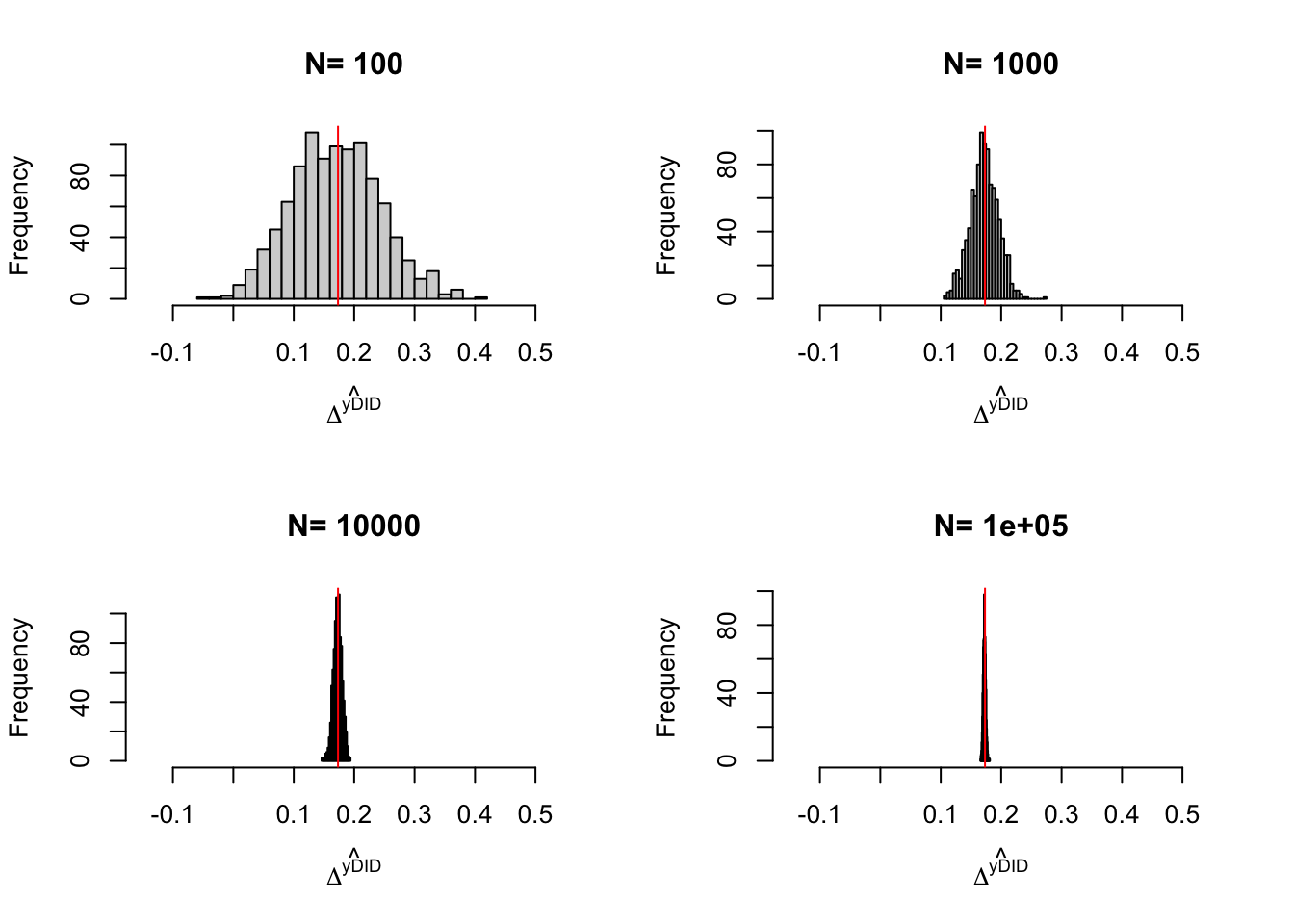
Figure 4.19: Distribution of the DID estimator over replications of panels of different sizes

Figure 4.19 shows that the DID estimator converges pretty fast to the true treatment effect as sample size grows large. Let us now wee what happens with a repeated cross section:

monte.carlo.did.cross <- function(s,N,param){
  N.tot <- 2*N
  set.seed(s)
  mu <- rnorm(N.tot,param["barmu"],sqrt(param["sigma2mu"]))
  UB <- rnorm(N.tot,0,sqrt(param["sigma2U"]))
  yB <- mu + UB 
  YB <- exp(yB)
  Ds <- rep(0,N.tot)
  Ds[YB<=param["barY"]] <- 1 
  epsilon <- rnorm(N.tot,0,sqrt(param["sigma2epsilon"]))
  eta<- rnorm(N.tot,0,sqrt(param["sigma2eta"]))
  U0 <- param["rho"]*UB + epsilon
  y0 <- mu +  U0 + param["delta"]
  alpha <- param["baralpha"]+  param["theta"]*mu + eta
  y1 <- y0+alpha
  Y0 <- exp(y0)
  Y1 <- exp(y1)
  y <- y1*Ds+y0*(1-Ds)
  Y <- Y1*Ds+Y0*(1-Ds)
  # first cross section: 1-N
  first <- seq(1,N)
  # second cross section: 1001-2000
  second <- seq(N+1,N.tot)
  # repeated cross section DID
  delta.y.did.cross <- mean(y[second][Ds[second]==1])-mean(y[second][Ds[second]==0])-(mean(yB[first][Ds[first]==1])-mean(yB[first][Ds[first]==0]))
  return(delta.y.did.cross)
}

simuls.did.cross.N <- function(N,Nsim,param){
  simuls.did.cross <- matrix(unlist(lapply(1:Nsim,monte.carlo.did.cross,N=N,param=param)),nrow=Nsim,ncol=1,byrow=TRUE)
  colnames(simuls.did.cross) <- c('DID')
  return(simuls.did.cross)
}

sf.simuls.did.cross.N <- function(N,Nsim,param){
  sfInit(parallel=TRUE,cpus=8)
  sim <- matrix(unlist(sfLapply(1:Nsim,monte.carlo.did.cross,N=N,param=param)),nrow=Nsim,ncol=1,byrow=TRUE)
  sfStop()
  colnames(sim) <- c('DID')
  return(sim)
}

Nsim <- 1000
#Nsim <- 10
N.sample <- c(100,1000,10000,100000)
#N.sample <- c(100,1000,10000)
#N.sample <- c(100,1000)
#N.sample <- c(100)

simuls.did.cross <- lapply(N.sample,sf.simuls.did.cross.N,Nsim=Nsim,param=param)
names(simuls.did.cross) <- N.sample

Let us now plot the results:

par(mfrow=c(2,2))
for (i in 1:length(simuls.did.cross)){
  hist(simuls.did.cross[[i]][,'DID'],breaks=30,main=paste('N=',as.character(N.sample[i])),xlab=expression(hat(Delta^yDID)),xlim=c(-0.15,0.55))
  abline(v=TT.pop,col="red")
}

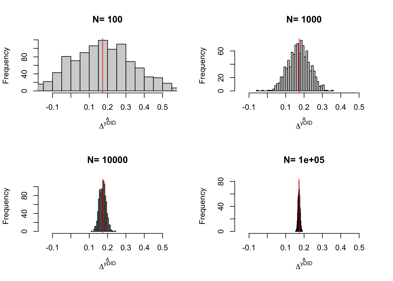
Figure 4.20: Distribution of the DID estimator over replications of repeated cross sections of different sizes

Relative to Figure 4.19, Figure 4.20 shows that sampling noise is larger at each sample size with a repeated cross section estimator. Let’s see how we can estimate these below using the Central Limit Theorem.

4.3.1.3 Estimation of sampling noise

It is especially important to understand the properties of sampling noise for treatment effect estimators in DID designs because it can serve as a basis for power analysis, but also to understand the sources of improvements or loss of precision when moving from the simple with/without comparison to the DID estimator. Let us first look at the sampling noise of the simpler $2\times 2$ DID estimator in a panel data with only two time periods. We will then move to the sampling noise of the simpler $2\times 2$ DID estimator in a repeated cross section.

4.3.1.3.1 Estimating sampling noise in panel settings

When we estimate DID in a panel of two time periods, Theorem 4.10 shows that all possible DID estimators are equivalent. We can thus use the most convenient one in order to derive the Central Limit Theorem-based approximation to its distribution, and use it to estimate sampling noise. The most convenient estimator, to me, is the First Difference estimator. We indeed know that it is formulated as an OLS estimator, regressing the change in outcomes over time to the treatment dummy. The First Difference estimator is thus simply a With/Without estimator where the outcomes are replaced by the changes in outcomes over time. And we already know how to derive an Central Limit Theorem-based estimate of the sampling noise of the With/Without estimator. In order to use these results, we need some assumptions:

Hypothesis 4.15 (i.i.d. sampling in First Difference) We assume that the observations in the sample are identically and independently distributed in First Differences: \[\begin{align*} \forall i,j\leq N\text{, }i\neq j\text{, } & (Y_{i,A}-Y_{i,B},D_i)\Ind(Y_{j,A}-Y_{j,B},D_j),\\ & (Y_{i,A}-Y_{i,B},D_i)\&(Y_{j,A}-Y_{j,B},D_j)\sim F_{Y_A-Y_B,D}. \end{align*}\]

Assumption 4.15 imposes that the changes in outcome over time are not correlated across units. This is not a strong assumption. It is actually much weaker than imposing that the levels of outcomes are distributed i.i.d. in the sample. That would require that the outcomes of the same unit are not correlated over time, which is wrong if there are unit fixed effects $\mu_i$ or if the error terms are correlated across time (which is possible if shocks are persistent). Assumption 4.15 rules out spatial correlation between units, be it in the changes in outcomes or in receiving the treatment. This is very restrictive.

We also need to assume that the changes in outcomes in both groups have finite variances:

Hypothesis 4.16 (Finite variance of $\hat{\Delta^Y_{WW}}$) We assume that $\var{Y^1_A-Y^0_B|D_i=1}$ and $\var{Y^0_A-Y^0_B|D_i=0}$ are finite.

We now can state the following theorem:

Theorem 4.11 (Asymptotic Distribution of the DID Estimator in Panel Data) Under Assumptions 4.12, 4.13, 4.14, 4.15 and 4.16, we have:

\[\begin{align*} \sqrt{N}(\hat{\Delta}^Y_{DID}-\Delta^Y_{DID}) & \stackrel{d}{\rightarrow} \mathcal{N}\left(0,\frac{\var{Y_{i,A}^1-Y_{i,B}^0|D_i=1}}{\Pr(D_i=1)}+\frac{\var{Y_{i,A}^0-Y_{i,B}^0|D_i=0}}{1-\Pr(D_i=1)}\right). \end{align*}\]

Proof. Under Assumptions 4.12, 4.13, 4.14, Theorem 4.10 proves that $\hat{\Delta}^Y_{DID}=\hat{\beta}^{FD}$. $\hat{\beta}^{FD}$ is obtained as the OLS estimator of the coefficient in front of $D_i$ in a regression of $Y_{i,A}-Y_{i,B}$ on $D_i$ and a constant. Lemma A.3 shows that, in such a regression, this coefficient is also a WW estimator, so that $\hat{\beta}^{FD}=\hat{\Delta}^{Y_{A}-Y_{B}}_{WW}$. Using Theorem 2.5 proves the result.

Theorem 4.11 shows that the precision of the DID estimator in panel settings depends on the variance of the changes in outcomes over time in the treated and control group. Since outcomes for a given individual are generally correlated over time, the variance of the DID estimator will in general be lower than the variance of the WW estimator. A case in point is when there are individual fixed effects in the equation generating outcomes: in that case, differencing outcomes over time gets rid of the individual fixed effects and thus the variance of the differences out outcomes is lower than the variance of outcomes in levels, since it misses the part due to the individual fixed effects. So, in most cases (but not all of them), we can expect an increase in precision when moving from WW to DID.

Example 4.35 Let’s see how our estimator of sampling noise performs in the data.

The true level of 99% sampling noise in the $N=$ 1000 sample is estimated from the simulations to be equal to 0.12, while the estimated level of 99% sampling noise using the formula from Theorem 4.11 is equal to 0.1. The estimated level of 99% sampling noise obtained using the heteroskedasticity robust standard errors from the First Difference regression using OLS is equal to 0.11. The estimated level of 99% sampling noise obtained using the heteroskedasticity robust standard errors from the DID regression using OLS is equal to 0.34. It is much larger, because it assumes that we only have access to a repeated cross section, and thus it does not take into account the fact that we have more precision thanks to the panel data. The estimated level of 99% sampling noise obtained using the heteroskedasticity robust standard errors from the Within regression using OLS is equal to 0.08. The plm package corrects all standard errors for the panel nature of the data (irrespective of the type of estimator), and thus returns an estimate of 99% sampling noise equal to 0.11 for the Within estimator, 0.11 for the First Difference estimator and 0.11 for the pooled DID estimator. Neither lfe nor fixest seem compatible with vcovHC, which enables the estimation of heteroskedasticity-robust standard errors. The lfe package seems not to take into account heteroskedasticity by default: its estimate of 99% sampling noise is equal to 0.1. The fixest package seems to take into account heteroskedasticity by default: its estimate of 99% sampling noise is equal to 0.11.

4.3.1.3.2 Estimating sampling noise in repeated cross sections

When we do not have access to panel data, a lot of the estimators we have studied here are infeasible. This is the case of the First Difference estimator (we cannot build the difference in out comes over time for the same unit since we observe each unit only once). The Within estimator is also compromised (we cannot build the average outcome over time for each observation, since, again, we only observe each observation only once). The Least Squares Dummy Variables estimator is also infeasible, for the same reason: we need to observe each observation at least twice in order for the treatment dummy to not be collinear with the unit and time fixed effects.

But, both the basic DID formula and the Least Squares pooling estimator can still be computed with repeated cross sections. As Figure 4.20 has shown, the DID estimator is much more variable in repeated cross section: the level of 99% sampling noise in the $N=$ 1000 sample is estimated from the simulations to be equal to 0.28, while it is of 0.12 with panel data of the same size. Let’s see how the Central-Limit Theorem can help us estimate this variance and shed some light on why we lose so much precision when moving from panel to cross section estimators. It is unfortunately much more work to derive the CLT-based estimate of sampling noise with repeated cross-sections than with panel data. We first need to respecify an i.i.d. assumption adapted to repeated cross sections:

Hypothesis 4.17 (i.i.d. sampling in Repeated Cross Sections) We assume that the observations in the sample are identically and independently distributed: \[\begin{align*} \forall i,j\leq N_t\text{, }i\neq j\text{, }, \forall t,t'\in\{A,B\}\text{, }t\neq t'\text{, } & (Y_{i,t},D_i)\Ind(Y_{j,t'},D_j),\\ & (Y_{i,t},D_i)\&(Y_{j,t'},D_j)\sim F_{Y,D}. \end{align*}\]

Assumption 4.17 imposes that outcomes are not correlated across units nor across time. This is not a strong assumption in a repeated cross section, as long as the same units are not observed at both periods. We now can state the following theorem:

Theorem 4.12 (Asymptotic Distribution of the DID Estimator in Repeated Cross Sections) Under Assumptions 4.12, 4.13, 4.14, 4.17 and 2.3, we have:

\[\begin{align*} \sqrt{N}(\hat{\Delta}^Y_{DID}-\Delta^Y_{DID}) & \stackrel{d}{\rightarrow} \mathcal{N}\left(0,\frac{\var{Y^0_{i,B}|D_i=0}}{(1-p)(1-p_A)} +\frac{\var{Y^0_{i,B}|D_i=1}}{p(1-p_A)}\right.\\ & \phantom{\stackrel{d}{\rightarrow}\mathcal{N}\left(0,\right.} \left. +\frac{\var{Y^0_{i,A}|D_i=0}}{(1-p)p_A} +\frac{\var{Y^1_{i,A}|D_i=1}}{pp_A}\right). \end{align*}\]

where $p=\Pr(D_i=1)$ and $p_A$ is the proportion of observations belonging to the After period.

Proof. See Section A.3.2.

Remark. Note that the difference between the amount of sampling noise of the DID estimator in panel data in repeated cross sections is present whatever the estimator (in panel data, all the estimators are equivalent). It is not differencing or taking the within transformation that gets rid of sampling noise, it is collecting data on the same observations twice. Differencing only helps the OLS estimator of the standard errors to understand that we have panel data and to reflect it in its estimate of precision. The DID estimator is always more precise in panel data (in our example). The CLT-based estimator of precision does not always reflect that fact, because we have not correctly specified it.

Example 4.36 Let’s see how our estimator of sampling noise performs in the data.

The true level of 99% sampling noise in the $N=$ 1000 sample is estimated from the simulations to be equal to 0.28, while the estimated level of 99% sampling noise using the formula from Theorem 4.12 is equal to 0.34. The estimated level of 99% sampling noise obtained using the heteroskedasticity robust standard errors from the DID regression using OLS is equal to 0.34.

4.3.2 Reverse Difference In Differences designs with two time periods

Before getting into the general case of DID with several time periods and several treatment dates, it is useful to quickly look at identification in the case of reverse DID designs. We are going to look at two such designs. In the first type, some units are exposed to the treatment in the first period and the rest of the units enter the treatment in the second period. In the second type of reverse DID design, all units receive the treatment in the first period and some units exit the treatment in the second period.

4.3.2.1 Reverse DID designs where everyone enters the treatment at the second period

Compared to the setting in the previous section, the main change is to Assumption 4.12:

Hypothesis 4.18 (Everyone Receives Treatment in the Second Period) We assume that every unit in the population receives the treatment in the second period: $D_{i,A}=1$, $\forall i$.

Under Assumption 4.18, and without loss of generality, we can write $D_i=D_{i,B}$, $\forall i$. We are going to call the units which stay in the treatment during the two periods always takers and the units who enter the treatment in the second period switchers. Always takers are defined by $D_i=1$ while switchers are defined by $D_i=0$.

In this new setting, we have to redefine the DID estimator. We are going to choose an estimator that compares the change in outcomes among individuals who have changed treatment status (switchers) to the change in outcome among individuals who have not changed treatment status (always takers):

\[\begin{align*} \Delta^Y_{DID^r} & = \esp{Y_{i,A}|D_i=0} - \esp{Y_{i,B}|D_i=0} - (\esp{Y_{i,A}|D_i=1} - \esp{Y_{i,B}|D_i=1}).\\ \end{align*}\]

Note that $\Delta^Y_{DID^r}$ is the opposite of the more usual DID estimator $\Delta^Y_{DID}$, hence the name of reverse DID.

Example 4.37 Let us generate data in our example model that complies with Assumption 4.18.

\[\begin{align*} y^1_{i,A} & = y_{i,A}^0+\bar{\alpha}_A+\bar{\alpha}_{AT}D_{i,B}+\theta_A\mu_i+\eta_{i,A} \\ y^0_{i,A} & = \mu_i+\delta+U^0_{i,A} \\ U^0_{i,A} & = \rho U_{i,B}+\epsilon_{i,A} \\ y^1_{i,B} & =y^0_{i,B} + \bar{\alpha}_B+\theta_B\mu_i+\eta_{i,B} \\ y^0_{i,B} & =\mu_i+U_{i,B} \\ U_{i,B} & \sim\mathcal{N}(0,\sigma^2_{U}) \\ D_{i,B} & = \uns{y^0_{i,B}+ V_i\leq\bar{y}} \\ V_i & = \gamma(\mu_i-\bar{\mu}) + \omega_i \\ (\eta_{i,A},\eta_{i,B},\omega_i) & \sim\mathcal{N}(0,0,0,\sigma^2_{\eta},\sigma^2_{\eta},\sigma^2_{\omega},0,\rho_{\eta,\omega}) \end{align*}\]

Note that in this model we first have imposed that some people enter the treatment in the first period (period $B$). We also have added other important features, such as the fact that the effect of the treatment varies over time. The most important component of this variation is the constant parameter $\bar{\alpha}$ which now differs from period to period ($\bar{\alpha}_A\neq\bar{\alpha}_B$). The treatment effect also varies over group and over time, with the always treated group (characterized by $D_{i,B}=1$) having an additional increase in treatment effects of $\bar{\alpha}_{AT}$ in period $A$. Let’s encode new parameter values.

param <- c(8,.5,.28,1500,0.9,0.01,0.01,0.05,0.05,0.05,0.2,0.1,0.3,0.1,0.28,0)
names(param) <- c("barmu","sigma2mu","sigma2U","barY","rho","thetaA","thetaB","sigma2epsilon","sigma2eta","delta","baralphaA","baralphaB","baralphaAT","gamma","sigma2omega","rhoetaomega")

Let’s now simulate a dataset according to these new equations.

set.seed(1234)
N <- 1000
cov.eta.omega <- matrix(c(param["sigma2eta"],0,param["rhoetaomega"]*sqrt(param["sigma2eta"]*param["sigma2omega"]),
                          0,param["sigma2eta"],param["rhoetaomega"]*sqrt(param["sigma2eta"]*param["sigma2omega"]),
                          param["rhoetaomega"]*sqrt(param["sigma2eta"]*param["sigma2omega"]),param["rhoetaomega"]*sqrt(param["sigma2eta"]*param["sigma2omega"]),param["sigma2omega"]),ncol=3,nrow=3,byrow=T)
eta.omega <- as.data.frame(mvrnorm(N,c(0,0,0),cov.eta.omega))
colnames(eta.omega) <- c('etaA','etaB','omega')
mu <- rnorm(N,param["barmu"],sqrt(param["sigma2mu"]))
UB <- rnorm(N,0,sqrt(param["sigma2U"]))
y0B <- mu + UB 
Y0B <- exp(y0B)
Ds <- rep(0,N)
V <- param["gamma"]*(mu-param["barmu"])+eta.omega$omega
Ds[y0B+V<=log(param["barY"])] <- 1 
alphaB <- param["baralphaB"]+  param["thetaB"]*mu + eta.omega$etaB
y1B <- y0B+alphaB
Y1B <- exp(y1B)
epsilonA <- rnorm(N,0,sqrt(param["sigma2epsilon"]))
U0A <- param["rho"]*UB + epsilonA
y0A <- mu +  U0A + param["delta"]
alphaA <- param["baralphaA"]+ param["baralphaAT"]*Ds+ param["thetaA"]*mu + eta.omega$etaA
y1A <- y0A+alphaA
Y0A <- exp(y0A)
Y1A <- exp(y1A)
yB <- y1B*Ds+y0B*(1-Ds)
YB <- Y1B*Ds+Y0B*(1-Ds)
yA <- y1A
YA <- Y1A

Let’s see how DID works on this data.

x <- c("Before","After")
y.AT <- c(mean(yB[Ds==1]),mean(yA[Ds==1]))
y.AT.counterfactual <- c(mean(y0B[Ds==1]),mean(y0A[Ds==1]))
y.Switchers <- c(mean(yB[Ds==0]),mean(yA[Ds==0]))
y.Switchers.counterfactual <- c(mean(y0B[Ds==0]),mean(y0A[Ds==0]))
y.Switchers.counterfactual.1 <- c(mean(y1B[Ds==0]),mean(y1A[Ds==0]))
y.Switchers.DID <- c(mean(yB[Ds==0]),mean(yB[Ds==0])+mean(yA[Ds==1])-mean(yB[Ds==1]))
y.Switchers.DID.1 <- c(mean(yA[Ds==0])-(mean(yA[Ds==1])-mean(yB[Ds==1])),mean(yA[Ds==0]))
data.DID.plot <- as.data.frame(c(y.AT,y.AT.counterfactual,y.Switchers,y.Switchers.counterfactual,y.Switchers.counterfactual.1,y.Switchers.DID,y.Switchers.DID.1))
colnames(data.DID.plot) <- c("Outcome") 
data.DID.plot$Period <- factor(rep(x,7),levels=c("Before","After"))
data.DID.plot$Group <- factor(c("Always Treated","Always Treated","Always Treated counterfactual y0","Always Treated counterfactual y0","Switchers","Switchers","Switchers counterfactual y0","Switchers counterfactual y0","Switchers counterfactual y1","Switchers counterfactual y1","Switchers DIDr","Switchers DIDr","Switchers DIDr1","Switchers DIDr1"),levels=c("Switchers","Switchers counterfactual y1","Switchers counterfactual y0","Switchers DIDr","Switchers DIDr1","Always Treated","Always Treated counterfactual y0"))
data.DID.plot$Observed <- factor(c("Observed","Observed","Unobserved","Unobserved","Observed","Observed","Unobserved","Unobserved","Unobserved","Unobserved","Generated","Generated","Generated","Generated"),levels=c("Observed","Unobserved","Generated"))

WW.before <- (mean(yB[Ds==0])-mean(yB[Ds==1]))
WW.after <- (mean(yA[Ds==0])-mean(yA[Ds==1]))
BA.AT <- mean(yA[Ds==1])-mean(yB[Ds==1])
BA.Switchers <- mean(yA[Ds==0])-mean(yB[Ds==0])
Counterfactual.after <- mean(yB[Ds==0])+BA.AT
DIDr <- BA.Switchers - BA.AT 
TTASwitchers <- mean(alphaA[Ds==0])
TTBSwitchers <- mean(alphaB[Ds==0])
TTAAT <- mean(alphaA[Ds==1])
TTBAT <- mean(alphaB[Ds==1])

ggplot(data.DID.plot,aes(x=Period,y=Outcome,group=Group,color=Group,shape=Group,linetype=Observed))+
    geom_line() +
    geom_point()+
    scale_linetype_discrete(guide='none') +
    theme_bw()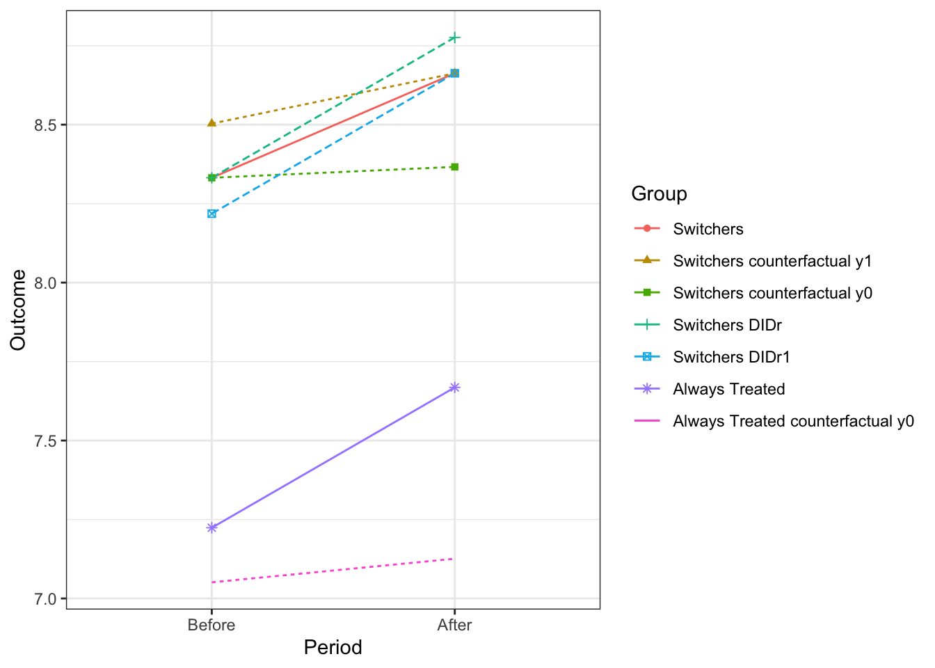

Evolution of average outcomes in the always treated and switchers group in the reverse DID design where everyone is treated in the second period

Figure 4.21: Evolution of average outcomes in the always treated and switchers group in the reverse DID design where everyone is treated in the second period

Figure 4.21 shows that DID does not work well in this example. Indeed, the true treatment effect among switchers after the treatment is equal to 0.3 in the sample, while the DID estimator is equal to -0.11. The $DID^r$ estimator is of the wrong sign. Why is that? Note that the $DID^r$ estimator uses the change in outcomes among the always treated to approximate the change in outcome that would have occurred for the switchers if they have stayed outside of the treatment. The problem is that this approximation does not work at all: the increases in outcome for the always treated is much steeper than the increase in outcomes that would have happened to the switchers had they stayed outside of the treatment (0.44 $>$ 0.33). As a consequence, the $DID^r$ estimator overestimates the counterfactual level that would have been reached by the switchers in the second period in the absence of the treatment. Ultimately, the $DID^r$ estimator underestimates severely the effect of the treatment. Note that the usual assumption of parallel trends does hold in this example. The problem comes form somewhere else. One way to understand the problems with the $DID^r$ estimator is to see that the change in treatment effects over time and between groups over time confounds the effect of the treatment. The only way to make the $DID^r$ estimator work is to assume these confounders away.

In order to clarify the conditions under which the $DID^r$ estimator is valid, let us state the following assumption:

Hypothesis 4.19 (Parallel Trends in the presence of the treatment) We assume that the trends in the potential outcomes in the presence the treatment are the same for the treated and the untreated units:

\[\begin{align*} \esp{Y^1_{i,A}|D_i=1} - \esp{Y^1_{i,B}|D_i=1} & = \esp{Y^1_{i,A}|D_i=0} - \esp{Y^1_{i,B}|D_i=0}. \end{align*}\]

Under Assumption 4.19, we can show that the $DID^r$ estimator identifies the effect of the treatment on the switchers in the first period:

Theorem 4.13 (DIDr identifies TUT in the first period) Under Assumptions 4.12, 4.13 and 4.19, the $DID^r$ estimator identifies the average effect of the Treatment on the switchers before the treatment:

\[\begin{align*} \Delta_{DID^r}^{Y} & = \Delta^{Y_B}_{TUT}, \end{align*}\]

with:

\[\begin{align*} \Delta^{Y_B}_{TUT} & = \esp{Y^1_{i,B}-Y^0_{i,B}|D_{i}=0}. \end{align*}\]

Proof. \[\begin{align*} \Delta^Y_{DID^r} & = \esp{Y_{i,A}|D_i=0}-\esp{Y_{i,B}|D_i=0}-(\esp{Y_{i,A}|D_i=1}-\esp{Y_{i,B}|D_i=1}) \\ & = \esp{Y^1_{i,A}|D_i=0}-\esp{Y^0_{i,B}|D_i=0}-(\esp{Y^1_{i,A}|D_i=1}-\esp{Y^1_{i,B}|D_i=1})\\ & = \esp{Y^1_{i,A}|D_i=0} - \esp{Y^0_{i,B}|D_i=0}-(\esp{Y^1_{i,A}|D_i=0}-\esp{Y^1_{i,B}|D_i=0})\\ & = \esp{Y^1_{i,B}-Y^0_{i,B}|D_i=0} \end{align*}\]

where the second equality follows from Assumptions 4.12 and 4.13 and the switching equation, and the third equality follows from Assumption 4.19.

Theorem 4.13 shows that under an alternative assumption of parallel trends (that they hold for potential outcomes when units are in the treatment), the $DID^r$ estimator identifies the causal effect of the treatment on the switchers before the treatment takes place.

Remark. Note that it makes intuitive sense: the only true change is that of the switchers entering the treatment. Using the always takers, we can only learn about the changes in potential outcomes when in the treatment. Under Assumption 4.19, the switchers would have experimented the same change in outcomes than the always takers if they have been constantly treated. As a consequence, we can use the change in outcomes among the always takers to project back what would have been the outcomes of the switchers in the first period had they been exposed to the treatment.

Remark. Note as well that Assumption 4.19, when paired with Assumption 4.14, is actually restrictive in terms of how the treatment effects might change over time and between groups, as the following lemma shows:

Lemma 4.4 (Parallel Trends Restricts the Way Treatment Effects Change Over Time) Assumptions 4.14 and 4.19 imply that always takers and switchers experience the same changes in treatment effects over time:

\[\begin{align*} \Delta^{Y_A}_{TUT}- \Delta^{Y_B}_{TUT} & = \Delta^{Y_A}_{TT}- \Delta^{Y_B}_{TT}. \end{align*}\]

Proof. Substracting the parallel trends condition in Assumption 4.14 from the parallel trends condition in Assumption 4.19, we have:

\[\begin{align*} \esp{Y^1_{i,A}|D_i=1} - \esp{Y^1_{i,B}|D_i=1}-(\esp{Y^0_{i,A}|D_i=1} - \esp{Y^0_{i,B}|D_i=1}) & = \esp{Y^1_{i,A}|D_i=0} - \esp{Y^1_{i,B}|D_i=0}-(\esp{Y^0_{i,A}|D_i=0} - \esp{Y^0_{i,B}|D_i=0}). \end{align*}\]

After some manipulation, we get:

\[\begin{align*} \esp{Y^1_{i,A}-Y^0_{i,A}|D_i=1} - \esp{Y^1_{i,B}-Y^0_{i,B}|D_i=1}& = \esp{Y^1_{i,A}-Y^0_{i,A}|D_i=0} - \esp{Y^1_{i,B}-Y^0_{i,B}|D_i=0},. \end{align*}\]

which proves the result.

Remark. There remains a final question: are there any conditions under which we could use the $DID^r$ estimator to identify the effect of the treatment on the switchers after the treatment takes place? In practice, that means that we need to recover the trends the switchers would have experienced had they not entered the treatment. This puts a stark requirement on the available data because we have no information on what outcomes in the absence of the treatment would be in the second period. One natural but also super strong assumption is to assume that the change in outcomes among the always takers in the presence of the treatment is the same as the one that the switchers would have experienced in the absence of the treatment:

Hypothesis 4.20 (Parallel Trends for Always Takers in the Presence of the Treatment and Switchers in the Absence of the Treatment) We assume that the trends in the potential outcomes in the presence the treatment for the always takers are the same as the trends in potential outcomes in the absence of the treatment for the switchers :

\[\begin{align*} \esp{Y^1_{i,A}|D_i=1} - \esp{Y^1_{i,B}|D_i=1} & = \esp{Y^0_{i,A}|D_i=0} - \esp{Y^0_{i,B}|D_i=0}. \end{align*}\]

Under Assumption 4.20, we can recover the treatment effect on teh switchers in the second period:

Theorem 4.14 (DIDr identifies TUT in the second period) Under Assumptions 4.12, 4.13 and 4.20, the $DID^r$ estimator identifies the average effect of the Treatment on the switchers after the treatment:

\[\begin{align*} \Delta_{DID^r}^{Y} & = \Delta^{Y_A}_{TUT}, \end{align*}\]

with:

\[\begin{align*} \Delta^{Y_A}_{TUT} & = \esp{Y^1_{i,A}-Y^0_{i,A}|D_{i}=0}. \end{align*}\]

Proof. \[\begin{align*} \Delta^Y_{DID^r} & = \esp{Y_{i,A}|D_i=0}-\esp{Y_{i,B}|D_i=0}-(\esp{Y_{i,A}|D_i=1}-\esp{Y_{i,B}|D_i=1}) \\ & = \esp{Y^1_{i,A}|D_i=0}-\esp{Y^0_{i,B}|D_i=0}-(\esp{Y^1_{i,A}|D_i=1}-\esp{Y^1_{i,B}|D_i=1})\\ & = \esp{Y^1_{i,A}|D_i=0} - \esp{Y^0_{i,B}|D_i=0}-(\esp{Y^0_{i,A}|D_i=0}-\esp{Y^0_{i,B}|D_i=0})\\ & = \esp{Y^1_{i,A}-Y^0_{i,A}|D_i=0} \end{align*}\]

where the second equality follows from Assumptions 4.12 and 4.13 and the switching equation, and the third equality follows from Assumption 4.20.

Remark. What does Assumption 4.20 really mean? It is unusual, but is it highly restrictive? The following lemma helps to make sense of it:

Lemma 4.5 (Parallel Trends and Treatment Effects) The parallel trends assumptions restrict the way treatment effects might change over time: (i) Assumptions 4.14 and 4.20 together imply the effect of the treatment is constant over time among always takers: $\Delta^{Y_A}_{TT} = \Delta^{Y_B}_{TT}$; (ii) Assumptions 4.19 and 4.20 together imply the effect of the treatment is constant over time among switchers: $\Delta^{Y_A}_{TUT} = \Delta^{Y_B}_{TUT}$; (iii) Assumptions 4.14, 4.19 and 4.20 together imply the effect of the treatment is constant over time among switchers and always takers: $\Delta^{Y_A}_{TUT} = \Delta^{Y_B}_{TUT}$ and $\Delta^{Y_A}_{TT} = \Delta^{Y_B}_{TT}$.

Proof. Substracting the parallel trends condition in Assumption 4.14 from the parallel trends condition in Assumption 4.20, we have:

\[\begin{align*} \esp{Y^1_{i,A}|D_i=1} - \esp{Y^1_{i,B}|D_i=1}-(\esp{Y^0_{i,A}|D_i=1} - \esp{Y^0_{i,B}|D_i=1}) & = \esp{Y^0_{i,A}|D_i=0} - \esp{Y^0_{i,B}|D_i=0}-(\esp{Y^0_{i,A}|D_i=0} - \esp{Y^0_{i,B}|D_i=0}). \end{align*}\]

After some manipulation, we get:

\[\begin{align*} \esp{Y^1_{i,A}-Y^0_{i,A}|D_i=1}& = \esp{Y^1_{i,B}-Y^0_{i,B}|D_i=1}. \end{align*}\]

which proves the first result.

Substracting the parallel trends condition in Assumption 4.19 from the parallel trends condition in Assumption 4.20, we have:

\[\begin{align*} \esp{Y^1_{i,A}|D_i=1} - \esp{Y^1_{i,B}|D_i=1}-(\esp{Y^1_{i,A}|D_i=1} - \esp{Y^1_{i,B}|D_i=1}) & = \esp{Y^1_{i,A}|D_i=0} - \esp{Y^1_{i,B}|D_i=0}-(\esp{Y^0_{i,A}|D_i=0} - \esp{Y^0_{i,B}|D_i=0}). \end{align*}\]

After some manipulation, we get:

\[\begin{align*} \esp{Y^1_{i,A}-Y^0_{i,A}|D_i=0}& = \esp{Y^1_{i,B}-Y^0_{i,B}|D_i=0}. \end{align*}\]

which proves the second result.

The first two results imply the last one.

Remark. It is noteworthy that combining the three assumptions together does not imply anything more than when combining them separately. The key is that Assumptions 4.14 and 4.19 together already imply that treatment effects change in the same way over time in both groups. Assumption 4.20 together with Assumptions 4.14 and 4.19 implies also that all potential outcomes have to change in the same way over time in both groups. The only way for these two properties to be true at the same time is for treatment effects in noth groups to be constant over time.

Remark. Note that Lemma 4.5 does not imply that treatment effects are the same in both groups. They do not have to be. Assumptions 4.14, 4.19 and 4.20 allow for the treatment effects among switchers and always takers to be different.

Remark. A useful result is also to express the bias of the $DID^r$ estimator when only Assumption 4.14 holds. The following lemma does the job:

Theorem 4.15 (Bias of the DIDr estimator) Under Assumptions 4.12, 4.13 and 4.14, the $DID^r$ estimator is biased for the average effect of the Treatment on the switchers before and after the treatment:

\[\begin{align*} \Delta_{DID^r}^{Y} & = \Delta^{Y_B}_{TUT}+B^{Y_B}_{DID^r} \\ \Delta_{DID^r}^{Y} & = \Delta^{Y_A}_{TUT}+B^{Y_A}_{DID^r} \end{align*}\]

with:

\[\begin{align*} B^{Y_B}_{DID^r} & = \Delta^{Y_A}_{TUT}-\Delta^{Y_B}_{TUT}-(\Delta^{Y_A}_{TT}-\Delta^{Y_B}_{TT})\\ B^{Y_A}_{DID^r} & = -(\Delta^{Y_A}_{TT}-\Delta^{Y_B}_{TT}). \end{align*}\]

Proof. \[\begin{align*} \Delta^Y_{DID^r} & = \esp{Y_{i,A}-Y_{i,B}|D_i=0}-\esp{Y_{i,A}-Y_{i,B}|D_i=1} \\ & = \esp{Y^1_{i,A}-Y^0_{i,B}|D_i=0}-\esp{Y^1_{i,A}-Y^1_{i,B}|D_i=1}\\ & = \esp{Y^1_{i,A}-Y^0_{i,B}|D_i=0}-\esp{Y^1_{i,A}-Y^1_{i,B}|D_i=0}+\esp{Y^1_{i,A}-Y^1_{i,B}|D_i=0}-\esp{Y^1_{i,A}-Y^1_{i,B}|D_i=1} \\ & = \esp{Y^1_{i,B}-Y^0_{i,B}|D_i=0}+\esp{Y^1_{i,A}-Y^1_{i,B}|D_i=0}-\esp{Y^1_{i,A}-Y^1_{i,B}|D_i=1} \\ & = \Delta^{Y_B}_{TUT}+\esp{Y^1_{i,A}-Y^1_{i,B}|D_i=0}-\esp{Y^1_{i,A}-Y^1_{i,B}|D_i=1}\\ & \phantom{=}-(\esp{Y^0_{i,A}-Y^0_{i,B}|D_i=0}-\esp{Y^0_{i,A}-Y^0_{i,B}|D_i=1})\\ & = \Delta^{Y_B}_{TUT}+\Delta^{Y_A}_{TUT}-\Delta^{Y_B}_{TUT}-(\Delta^{Y_A}_{TT}-\Delta^{Y_B}_{TT}) \end{align*}\]

where the second equality follows from Assumptions 4.12 and 4.13 and the switching equation, and the fifth equality follows from Assumption 4.14.

\[\begin{align*} \Delta^Y_{DID^r} & = \esp{Y_{i,A}-Y_{i,B}|D_i=0}-\esp{Y_{i,A}-Y_{i,B}|D_i=1} \\ & = \esp{Y^1_{i,A}-Y^0_{i,B}|D_i=0}-\esp{Y^1_{i,A}-Y^1_{i,B}|D_i=1}\\ & = \esp{Y^1_{i,A}-Y^0_{i,B}|D_i=0}-\esp{Y^0_{i,A}-Y^0_{i,B}|D_i=0}+\esp{Y^0_{i,A}-Y^0_{i,B}|D_i=0}\\ & \phantom{=}-\esp{Y^0_{i,A}-Y^0_{i,B}|D_i=1}+\esp{Y^0_{i,A}-Y^0_{i,B}|D_i=1}-\esp{Y^1_{i,A}-Y^1_{i,B}|D_i=1} \\ & = \esp{Y^1_{i,A}-Y^0_{i,A}|D_i=0}+\esp{Y^0_{i,A}-Y^0_{i,B}|D_i=1}-\esp{Y^1_{i,A}-Y^1_{i,B}|D_i=1} \\ & = \Delta^{Y_A}_{TUT}-(\esp{Y^1_{i,A}-Y^0_{i,A}|D_i=1}-\esp{Y^1_{i,B}-Y^0_{i,B}|D_i=1}) \\ & = \Delta^{Y_A}_{TUT}-(\Delta^{Y_A}_{TT}-\Delta^{Y_B}_{TT}) \end{align*}\]

where the second equality follows from Assumptions 4.12 and 4.13 and the switching equation, and the fourth equality follows from Assumption 4.14.

Theorem 4.15 helps to make sense of Figure 4.21. The bias of the $DID^r$ estimator for the average effect of the treatment on the switchers in the second period is equal to the opposite of the change in treatment effects for the always treated between the first and the second period. This means that if the effect of the treatment increases over time for the always takers, the $DID^r$ estimator will be biased negatively. If this negative bias is sufficiently large, it can make an altogether positive treatment effect (both on switchers and always takers at every period) look negative. This is a very serious problem and the main reason why you want to be very careful when using the $DID^r$ estimator. This is actually what happens in Figure 4.21: the change in treatment effect over time among the always treated is very large (it is equal to 0.37) while the treatment effect is only equal to 0.3. As a consequence, the $DID^r$ estimator is equal to -0.11 whereas every average treatment effect is positive: $\hat{\Delta}^{y_A}_{TT}=$ 0.54 $\hat{\Delta}^{y_B}_{TT}=$ 0.17, $\hat{\Delta}^{y_A}_{TUT}=$ 0.3 and $\hat{\Delta}^{y_B}_{TUT}=$ 0.17.

Theorem 4.15 also explains why the $DID^r$ estimator is biased for the effect of the treatment in the first period. This is because the effect of the treatment changes differently over time among switchers and among always takers. On Figure 4.21, the average treatment effect on switchers increases by 0.12, and it is not approximated well by the change in treatment effect among the always takers (0.37). As a consequence, the $DID^r$ estimator is equal to -0.11 while the average effect of the treatment on the switchers in the first period is equal to: $\hat{\Delta}^{y_B}_{TUT}=$ 0.17.

Example 4.38 Let us now explore how the way Theorem 4.15 plays out in our data. For that, we are going to first switch off the change in treatment effects that is specific to the always takers in the second period. As a case in point, we are going to set $\bar{\alpha}_{AT}=0$.

param["baralphaAT"] <- 0

Let’s now simulate a dataset according to these new equations.

set.seed(1234)
N <- 1000
cov.eta.omega <- matrix(c(param["sigma2eta"],0,param["rhoetaomega"]*sqrt(param["sigma2eta"]*param["sigma2omega"]),
                          0,param["sigma2eta"],param["rhoetaomega"]*sqrt(param["sigma2eta"]*param["sigma2omega"]),
                          param["rhoetaomega"]*sqrt(param["sigma2eta"]*param["sigma2omega"]),param["rhoetaomega"]*sqrt(param["sigma2eta"]*param["sigma2omega"]),param["sigma2omega"]),ncol=3,nrow=3,byrow=T)
eta.omega <- as.data.frame(mvrnorm(N,c(0,0,0),cov.eta.omega))
colnames(eta.omega) <- c('etaA','etaB','omega')
mu <- rnorm(N,param["barmu"],sqrt(param["sigma2mu"]))
UB <- rnorm(N,0,sqrt(param["sigma2U"]))
y0B <- mu + UB 
Y0B <- exp(y0B)
Ds <- rep(0,N)
V <- param["gamma"]*(mu-param["barmu"])+eta.omega$omega
Ds[y0B+V<=log(param["barY"])] <- 1 
alphaB <- param["baralphaB"]+  param["thetaB"]*mu + eta.omega$etaB
y1B <- y0B+alphaB
Y1B <- exp(y1B)
epsilonA <- rnorm(N,0,sqrt(param["sigma2epsilon"]))
U0A <- param["rho"]*UB + epsilonA
y0A <- mu +  U0A + param["delta"]
alphaA <- param["baralphaA"]+ param["baralphaAT"]*Ds+ param["thetaA"]*mu + eta.omega$etaA
y1A <- y0A+alphaA
Y0A <- exp(y0A)
Y1A <- exp(y1A)
yB <- y1B*Ds+y0B*(1-Ds)
YB <- Y1B*Ds+Y0B*(1-Ds)
yA <- y1A
YA <- Y1A

Let’s see how DID works on this data.

x <- c("Before","After")
y.AT <- c(mean(yB[Ds==1]),mean(yA[Ds==1]))
y.AT.counterfactual <- c(mean(y0B[Ds==1]),mean(y0A[Ds==1]))
y.Switchers <- c(mean(yB[Ds==0]),mean(yA[Ds==0]))
y.Switchers.counterfactual <- c(mean(y0B[Ds==0]),mean(y0A[Ds==0]))
y.Switchers.counterfactual.1 <- c(mean(y1B[Ds==0]),mean(y1A[Ds==0]))
y.Switchers.DID <- c(mean(yB[Ds==0]),mean(yB[Ds==0])+mean(yA[Ds==1])-mean(yB[Ds==1]))
y.Switchers.DID.1 <- c(mean(yA[Ds==0])-(mean(yA[Ds==1])-mean(yB[Ds==1])),mean(yA[Ds==0]))
data.DID.plot <- as.data.frame(c(y.AT,y.AT.counterfactual,y.Switchers,y.Switchers.counterfactual,y.Switchers.counterfactual.1,y.Switchers.DID,y.Switchers.DID.1))
colnames(data.DID.plot) <- c("Outcome") 
data.DID.plot$Period <- factor(rep(x,7),levels=c("Before","After"))
data.DID.plot$Group <- factor(c("Always Treated","Always Treated","Always Treated counterfactual y0","Always Treated counterfactual y0","Switchers","Switchers","Switchers counterfactual y0","Switchers counterfactual y0","Switchers counterfactual y1","Switchers counterfactual y1","Switchers DIDr","Switchers DIDr","Switchers DIDr1","Switchers DIDr1"),levels=c("Switchers","Switchers counterfactual y1","Switchers counterfactual y0","Switchers DIDr","Switchers DIDr1","Always Treated","Always Treated counterfactual y0"))
data.DID.plot$Observed <- factor(c("Observed","Observed","Unobserved","Unobserved","Observed","Observed","Unobserved","Unobserved","Unobserved","Unobserved","Generated","Generated","Generated","Generated"),levels=c("Observed","Unobserved","Generated"))

WW.before <- (mean(yB[Ds==0])-mean(yB[Ds==1]))
WW.after <- (mean(yA[Ds==0])-mean(yA[Ds==1]))
BA.AT <- mean(yA[Ds==1])-mean(yB[Ds==1])
BA.Switchers <- mean(yA[Ds==0])-mean(yB[Ds==0])
Counterfactual.after <- mean(yB[Ds==0])+BA.AT
DIDr <- BA.Switchers - BA.AT 
TTASwitchers <- mean(alphaA[Ds==0])
TTBSwitchers <- mean(alphaB[Ds==0])
TTAAT <- mean(alphaA[Ds==1])
TTBAT <- mean(alphaB[Ds==1])

ggplot(data.DID.plot,aes(x=Period,y=Outcome,group=Group,color=Group,shape=Group,linetype=Observed))+
    geom_line() +
    geom_point()+
    scale_linetype_discrete(guide='none') +
    theme_bw()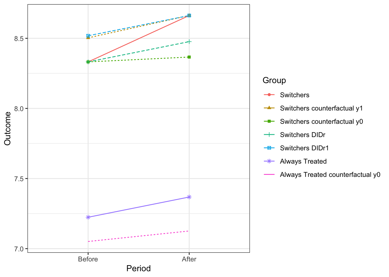

$Evolution of average outcomes in the always treated and switchers group in the reverse DID design where everyone is treated in the second period and $\bar{\alpha}_{AT}=0$$

Figure 4.22: Evolution of average outcomes in the always treated and switchers group in the reverse DID design where everyone is treated in the second period and $\bar{\alpha}_{AT}=0$

What is happening on Figure 4.22? First, the $DID^r$ estimator is equal to 0.19, while the effect of the treatment on switchers is equal to 0.3 in the second period and to 0.17 in the first period. So now, the bias of the $DID^r$ is not so large as to make it reverse signs with respect to the true effect of the treatment. It is actually almost zero for the effect on the switchers in the first period ($\hat{B}^{Y_B}_{DID^r}=$ 0.01). This is because the condition for $DID^r$ to capture the effect of the treatment on switchers in the first period is almost fulfilled in the data. Theorem 4.15 shows that this bias is equal to the difference in the change in teatment effect over time between the switchers and the always takers. The change in treatment effect for the switchers is equal to $\hat{\Delta}^{Y_A}_{TUT}-\hat\Delta^{Y_B}_{TUT}=$ 0.12 and the change in treatment effect for the always takers is equal to $\hat{\Delta}^{Y_A}_{TT}-\hat\Delta^{Y_B}_{TT}=$ 0.07. They are almost equal which makes $DID^r$ almost unbiased for the effect of the treatment on switchers in the first period.

On the contrary, the condition for $DID^r$ to capture the effect of the treatment on the switchers in the second period is not fulfilled in the data, not even almost. Theorem 4.15 shows that the condition for $DID^r$ to capture the effect of the treatment on the switchers in the second period is that the treatment effect on always takers be constant over time. This is unfortunately not the case in this data, since $\hat{\Delta}^{Y_A}_{TT}-\hat\Delta^{Y_B}_{TT}=$ 0.07. The bias of the $DID^r$ estimator is thus large (and negative) for $\hat{\Delta}^{Y_A}_{TUT}$: $\hat{B}^{Y_A}_{DID^r}=$ -0.11.

Remark. Note that in this model, the $DID^r$ estimator is still biased for $\Delta^{Y_B}_{TUT}$. The reasons why are left as an exercise.

Example 4.39 Let us finally explore the last condition in Theorem 4.15 that makes $DID^r$ unbiased for $\Delta^{Y_A}_{TUT}$, the effect of the treatment on switchers in the second period. We are going to switch off the change in treatment effects that occurs over time in both groups: we are going to set $\bar{\alpha}_{A}=\bar{\alpha}_{B}=0.1$.

param["baralphaA"] <- 0.1
param["baralphaB"] <- 0.1

Let’s now simulate a dataset according to these new equations.

set.seed(1234)
N <- 1000
cov.eta.omega <- matrix(c(param["sigma2eta"],0,param["rhoetaomega"]*sqrt(param["sigma2eta"]*param["sigma2omega"]),
                          0,param["sigma2eta"],param["rhoetaomega"]*sqrt(param["sigma2eta"]*param["sigma2omega"]),
                          param["rhoetaomega"]*sqrt(param["sigma2eta"]*param["sigma2omega"]),param["rhoetaomega"]*sqrt(param["sigma2eta"]*param["sigma2omega"]),param["sigma2omega"]),ncol=3,nrow=3,byrow=T)
eta.omega <- as.data.frame(mvrnorm(N,c(0,0,0),cov.eta.omega))
colnames(eta.omega) <- c('etaA','etaB','omega')
mu <- rnorm(N,param["barmu"],sqrt(param["sigma2mu"]))
UB <- rnorm(N,0,sqrt(param["sigma2U"]))
y0B <- mu + UB 
Y0B <- exp(y0B)
Ds <- rep(0,N)
V <- param["gamma"]*(mu-param["barmu"])+eta.omega$omega
Ds[y0B+V<=log(param["barY"])] <- 1 
alphaB <- param["baralphaB"]+  param["thetaB"]*mu + eta.omega$etaB
y1B <- y0B+alphaB
Y1B <- exp(y1B)
epsilonA <- rnorm(N,0,sqrt(param["sigma2epsilon"]))
U0A <- param["rho"]*UB + epsilonA
y0A <- mu +  U0A + param["delta"]
alphaA <- param["baralphaA"]+ param["baralphaAT"]*Ds+ param["thetaA"]*mu + eta.omega$etaA
y1A <- y0A+alphaA
Y0A <- exp(y0A)
Y1A <- exp(y1A)
yB <- y1B*Ds+y0B*(1-Ds)
YB <- Y1B*Ds+Y0B*(1-Ds)
yA <- y1A
YA <- Y1A

Let’s see how DID works on this data.

x <- c("Before","After")
y.AT <- c(mean(yB[Ds==1]),mean(yA[Ds==1]))
y.AT.counterfactual <- c(mean(y0B[Ds==1]),mean(y0A[Ds==1]))
y.Switchers <- c(mean(yB[Ds==0]),mean(yA[Ds==0]))
y.Switchers.counterfactual <- c(mean(y0B[Ds==0]),mean(y0A[Ds==0]))
y.Switchers.counterfactual.1 <- c(mean(y1B[Ds==0]),mean(y1A[Ds==0]))
y.Switchers.DID <- c(mean(yB[Ds==0]),mean(yB[Ds==0])+mean(yA[Ds==1])-mean(yB[Ds==1]))
y.Switchers.DID.1 <- c(mean(yA[Ds==0])-(mean(yA[Ds==1])-mean(yB[Ds==1])),mean(yA[Ds==0]))
data.DID.plot <- as.data.frame(c(y.AT,y.AT.counterfactual,y.Switchers,y.Switchers.counterfactual,y.Switchers.counterfactual.1,y.Switchers.DID,y.Switchers.DID.1))
colnames(data.DID.plot) <- c("Outcome") 
data.DID.plot$Period <- factor(rep(x,7),levels=c("Before","After"))
data.DID.plot$Group <- factor(c("Always Treated","Always Treated","Always Treated counterfactual y0","Always Treated counterfactual y0","Switchers","Switchers","Switchers counterfactual y0","Switchers counterfactual y0","Switchers counterfactual y1","Switchers counterfactual y1","Switchers DIDr","Switchers DIDr","Switchers DIDr1","Switchers DIDr1"),levels=c("Switchers","Switchers counterfactual y1","Switchers counterfactual y0","Switchers DIDr","Switchers DIDr1","Always Treated","Always Treated counterfactual y0"))
data.DID.plot$Observed <- factor(c("Observed","Observed","Unobserved","Unobserved","Observed","Observed","Unobserved","Unobserved","Unobserved","Unobserved","Generated","Generated","Generated","Generated"),levels=c("Observed","Unobserved","Generated"))

WW.before <- (mean(yB[Ds==0])-mean(yB[Ds==1]))
WW.after <- (mean(yA[Ds==0])-mean(yA[Ds==1]))
BA.AT <- mean(yA[Ds==1])-mean(yB[Ds==1])
BA.Switchers <- mean(yA[Ds==0])-mean(yB[Ds==0])
Counterfactual.after <- mean(yB[Ds==0])+BA.AT
DIDr <- BA.Switchers - BA.AT 
TTASwitchers <- mean(alphaA[Ds==0])
TTBSwitchers <- mean(alphaB[Ds==0])
TTAAT <- mean(alphaA[Ds==1])
TTBAT <- mean(alphaB[Ds==1])

ggplot(data.DID.plot,aes(x=Period,y=Outcome,group=Group,color=Group,shape=Group,linetype=Observed))+
    geom_line() +
    geom_point()+
    scale_linetype_discrete(guide='none') +
    theme_bw()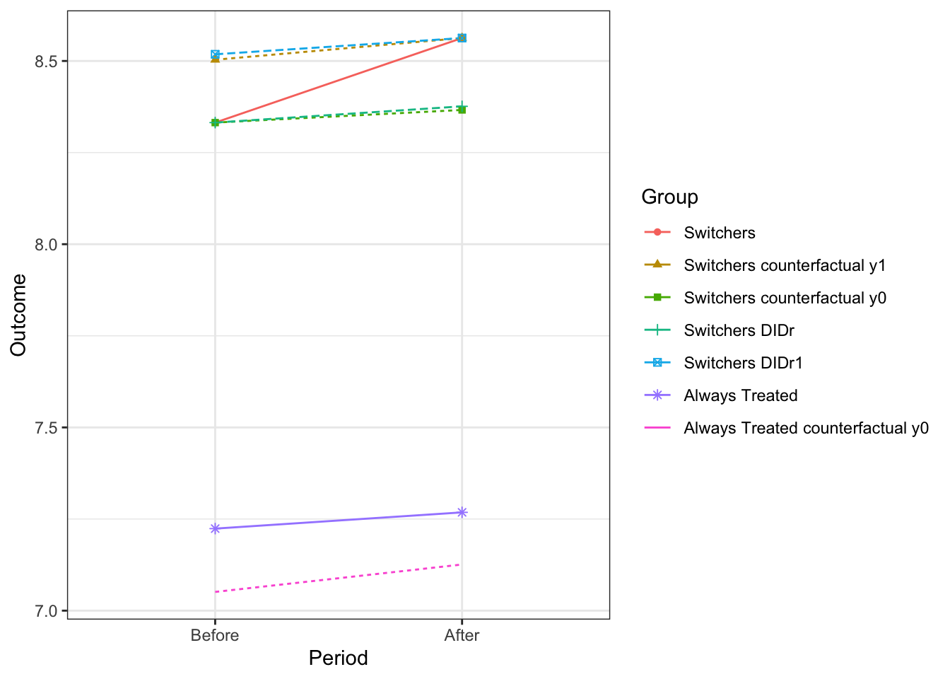

$Evolution of average outcomes in the always treated and switchers group in the reverse DID design where everyone is treated in the second period and $\bar{\alpha}_{A}=\bar{\alpha}_{B}=0$$

Figure 4.23: Evolution of average outcomes in the always treated and switchers group in the reverse DID design where everyone is treated in the second period and $\bar{\alpha}_{A}=\bar{\alpha}_{B}=0$

Figure 4.23 shows that the $DID^r$ estimator is almost OK in our setting. The $DID^r$ estimator is equal to 0.19 while the treatment effect on the switchers is equal to $\hat\Delta^{Y_A}_{TUT}=$ 0.2 in the second period and $\hat\Delta^{Y_B}_{TUT}=$ 0.17 in the first period. There still is a difference between the estimator and the treatment effect of interest, but the difference is small enough that it might be attributed to sampling noise. Remember that the condition for $DID^r$ to identify $\Delta^{Y_A}_{TUT}$ is Assumption 4.20 that the trends in potential outcomes in the absence of the treatment among switchers is the same as the trend in potential outcomes in the presence of the treatment among always takers. This is almost what we see, since the change in potential outcomes absent the treatment among switchers is equal to 0.03 while the change in potential outcomes under the treatment regime among always takers is equal to 0.04. The fact that these two quantities differ slightly is what biases the $DID^r$ estimator in the sample that we have generated. Note finally that Assumption 4.20 together with Assumption 4.14 implies that the effect of the treatment is constant over time among always takers, as Lemma 4.5 shows. This is also the condition for the $DID^r$ estimator to identify $\Delta^{Y_A}_{TUT}$ under Assumption 4.14, as Lemma 4.5 shows. Here, the effect of the treatment among always takers is equal to 0.17 in the first period and to 0.14 in the second period.

Remark. Actually, the conditions for $DID^r$ to indentify any treatment effect are not fulfilled in our model. That reasons why are left as an exercise.

4.3.2.2 DID designs where everyone is in the treatment at the first period

Compared to the setting in the previous section, the main change is to Assumption 4.12:

Hypothesis 4.21 (Everyone Receives Treatment in the First Period) We assume that every unit in the population receives the treatment in the first period: $D_{i,B}=1$, $\forall i$.

Under Assumption 4.21, and without loss of generality, we can still write $D_i=D_{i,A}$. In order for the $DID$ estimator to identify a fully-fledged treatment effect, we are going to need a pretty stark assumption:

Hypothesis 4.22 (No Effect After Exiting the Treatment) We assume that, after exiting the treatment, agents experience the same outcomes as if they had never entered the treatment: $Y_{i,A}=Y^0_{i,A}$, $\forall i$ such that $D_{i,A}=0$.

A consequence of Assumptions 4.21 and 4.22 is that we can write observed outcomes as a function of treatment and potential outcomes using the usual switching equation.

Remark. Note that Assumption 4.22 is extremely restrictive: units return immediately to their outcomes in the absence of the treatment right after exiting the treatment state. We are going to relax that assumption later.

The following theorem shows that $DID$ identifies a fully-fledged treatment effect under (arguably strong) assumptions:

Theorem 4.16 (DID identifies TUT in the second period) Under Assumptions 4.21, 4.22 and 4.19, the $DID$ estimator identifies the effect of the treatment on the switchers in the second period:

\[\begin{align*} \Delta_{DID}^{Y} & = \Delta^{Y_A}_{TUT}, \end{align*}\]

Proof. \[\begin{align*} \Delta^Y_{DID} & = \esp{Y_{i,A}|D_i=1}-\esp{Y_{i,B}|D_i=1}-(\esp{Y_{i,A}|D_i=0}-\esp{Y_{i,B}|D_i=0}) \\ & = \esp{Y^1_{i,A}|D_i=1}-\esp{Y^1_{i,B}|D_i=1}-(\esp{Y^0_{i,A}|D_i=0}-\esp{Y^1_{i,B}|D_i=0})\\ & = \esp{Y^1_{i,A}|D_i=0}-\esp{Y^1_{i,B}|D_i=0}-(\esp{Y^0_{i,A}|D_i=0}-\esp{Y^1_{i,B}|D_i=0})\\ & = \esp{Y^1_{i,A}-Y^0_{i,A}|D_i=0} \end{align*}\]

where the second equality follows from Assumptions 4.21 and 4.22 and the switching equation, and the third equality follows from Assumption 4.19.

Invoking another (even stronger) assumption, DID identifies the effect of the treatment on switchers in the first period:

Theorem 4.17 (DID identifies TUT in the first period) Under Assumptions 4.21, 4.22 and 4.20, the $DID$ estimator identifies the effect of the treatment on the switchers in the first period:

\[\begin{align*} \Delta_{DID}^{Y} & = \Delta^{Y_B}_{TUT}, \end{align*}\]

Proof. \[\begin{align*} \Delta^Y_{DID} & = \esp{Y_{i,A}|D_i=1}-\esp{Y_{i,B}|D_i=1}-(\esp{Y_{i,A}|D_i=0}-\esp{Y_{i,B}|D_i=0}) \\ & = \esp{Y^1_{i,A}|D_i=1}-\esp{Y^1_{i,B}|D_i=1}-(\esp{Y^0_{i,A}|D_i=0}-\esp{Y^1_{i,B}|D_i=0})\\ & = \esp{Y^0_{i,A}|D_i=0}-\esp{Y^0_{i,B}|D_i=0}-(\esp{Y^0_{i,A}|D_i=0}-\esp{Y^1_{i,B}|D_i=0})\\ & = \esp{Y^1_{i,B}-Y^0_{i,B}|D_i=0} \end{align*}\]

where the second equality follows from Assumptions 4.21 and 4.22 and the switching equation, and the third equality follows from Assumption 4.20.

We can also study the bias of the DID estimator under the classical parallel trends assumption (Assumption 4.14):

Lemma 4.6 (Bias of the DID estimator) Under Assumptions 4.21, 4.22 and 4.14, the $DID$ estimator is biased for the average effect of the Treatment on the switchers before and after the treatment:

\[\begin{align*} \Delta_{DID}^{Y} & = \Delta^{Y_B}_{TUT}+B^{Y_B}_{DID} \\ \Delta_{DID}^{Y} & = \Delta^{Y_A}_{TUT}+B^{Y_A}_{DID} \end{align*}\]

with:

\[\begin{align*} B^{Y_B}_{DID} & = \Delta^{Y_A}_{TT}-\Delta^{Y_B}_{TT}\\ B^{Y_A}_{DID} & = \Delta^{Y_A}_{TT}-\Delta^{Y_B}_{TT}-(\Delta^{Y_A}_{TUT}-\Delta^{Y_B}_{TUT}). \end{align*}\]

Proof. \[\begin{align*} \Delta^Y_{DID} & = \esp{Y_{i,A}-Y_{i,B}|D_i=1}-\esp{Y_{i,A}-Y_{i,B}|D_i=0} \\ & = \esp{Y^1_{i,A}-Y^1_{i,B}|D_i=1}-\esp{Y^0_{i,A}-Y^1_{i,B}|D_i=0}\\ & = \esp{Y^1_{i,A}-Y^1_{i,B}|D_i=1}-\esp{Y^0_{i,A}-Y^0_{i,B}|D_i=1}+\esp{Y^0_{i,A}-Y^0_{i,B}|D_i=0}-\esp{Y^0_{i,A}-Y^1_{i,B}|D_i=0} \\ & = \esp{Y^1_{i,B}-Y^0_{i,B}|D_i=0}+ \esp{Y^1_{i,A}-Y^1_{i,B}-(Y^0_{i,A}-Y^0_{i,B})|D_i=1} & = \Delta^{Y_B}_{TUT}+\Delta^{Y_A}_{TT}-\Delta^{Y_B}_{TT}, \end{align*}\]

where the second equality follows from Assumptions 4.21, 4.22 and the switching equation, and the third equality follows from Assumption 4.14.

\[\begin{align*} \Delta^Y_{DID} & = \esp{Y_{i,A}-Y_{i,B}|D_i=1}-\esp{Y_{i,A}-Y_{i,B}|D_i=0} \\ & = \esp{Y^1_{i,A}-Y^1_{i,B}|D_i=1}-\esp{Y^0_{i,A}-Y^1_{i,B}|D_i=0}\\ & = \esp{Y^1_{i,A}-Y^1_{i,B}|D_i=1}-\esp{Y^1_{i,A}-Y^1_{i,B}|D_i=0}+\esp{Y^1_{i,A}-Y^1_{i,B}|D_i=0}-\esp{Y^0_{i,A}-Y^1_{i,B}|D_i=0}\\ & = \esp{Y^1_{i,A}-Y^0_{i,A}|D_i=0}+\esp{Y^1_{i,A}-Y^1_{i,B}|D_i=1}-\esp{Y^1_{i,A}-Y^1_{i,B}|D_i=0} \\ & = \Delta^{Y_A}_{TUT}+\esp{Y^1_{i,A}-Y^1_{i,B}|D_i=1}-\esp{Y^1_{i,A}-Y^1_{i,B}|D_i=0}\\ & \phantom{=} -\esp{Y^0_{i,A}-Y^0_{i,B}|D_i=1}+\esp{Y^0_{i,A}-Y^0_{i,B}|D_i=0} \\ & = \Delta^{Y_A}_{TUT}+\Delta^{Y_A}_{TT}-\Delta^{Y_B}_{TT}-(\Delta^{Y_A}_{TUT}-\Delta^{Y_B}_{TUT}), \end{align*}\]

where the second equality follows from Assumptions 4.21, 4.22 and the switching equation, and the fifth equality follows from Assumption 4.14.

Example 4.40 Let us generate data in our example model that complies with Assumptions 4.21 and 4.22.

\[\begin{align*} y_{i,A}^1 & = y_{i,A}^0+\bar{\alpha}_A+\bar{\alpha}_{AT}D_{i,A}+\theta_A\mu_i+\eta_{i,A} \\ y_{i,A}^0 & = \mu_i+\delta+U_{i,A}^0 \\ U_{i,A}^0 & = \rho U_{i,B}+\epsilon_{i,A} \\ y^1_{i,B} & =y^0_{i,B} + \bar{\alpha}_B+\theta_B\mu_i+\eta_{i,B} \\ y^0_{i,B} & =\mu_i+U_{i,B} \\ U_{i,B} & \sim\mathcal{N}(0,\sigma^2_{U}) \\ D_{i,A} & = \uns{y^0_{i,B}+ V_i\leq\bar{y}} \\ V_i & = \gamma(\mu_i-\bar{\mu}) + \omega_i \\ (\eta_{i,A},\eta_{i,B},\omega_i) & \sim\mathcal{N}(0,0,0,\sigma^2_{\eta},\sigma^2_{\eta},\sigma^2_{\omega},0,\rho_{\eta,\omega}) \end{align*}\]

param <- c(8,.5,.28,1500,0.9,0.01,0.01,0.05,0.05,0.05,0.2,0.1,0.3,0.1,0.28,0)
names(param) <- c("barmu","sigma2mu","sigma2U","barY","rho","thetaA","thetaB","sigma2epsilon","sigma2eta","delta","baralphaA","baralphaB","baralphaAT","gamma","sigma2omega","rhoetaomega")

set.seed(1234)
N <- 1000
cov.eta.omega <- matrix(c(param["sigma2eta"],0,param["rhoetaomega"]*sqrt(param["sigma2eta"]*param["sigma2omega"]),
                          0,param["sigma2eta"],param["rhoetaomega"]*sqrt(param["sigma2eta"]*param["sigma2omega"]),
                          param["rhoetaomega"]*sqrt(param["sigma2eta"]*param["sigma2omega"]),param["rhoetaomega"]*sqrt(param["sigma2eta"]*param["sigma2omega"]),param["sigma2omega"]),ncol=3,nrow=3,byrow=T)
eta.omega <- as.data.frame(mvrnorm(N,c(0,0,0),cov.eta.omega))
colnames(eta.omega) <- c('etaA','etaB','omega')
mu <- rnorm(N,param["barmu"],sqrt(param["sigma2mu"]))
UB <- rnorm(N,0,sqrt(param["sigma2U"]))
y0B <- mu + UB 
Y0B <- exp(y0B)
Ds <- rep(0,N)
V <- param["gamma"]*(mu-param["barmu"])+eta.omega$omega
Ds[y0B+V<=log(param["barY"])] <- 1 
alphaB <- param["baralphaB"]+  param["thetaB"]*mu + eta.omega$etaB
y1B <- y0B+alphaB
Y1B <- exp(y1B)
epsilonA <- rnorm(N,0,sqrt(param["sigma2epsilon"]))
U0A <- param["rho"]*UB + epsilonA
y0A <- mu +  U0A + param["delta"]
alphaA <- param["baralphaA"]+ param["baralphaAT"]*Ds+ param["thetaA"]*mu + eta.omega$etaA
y1A <- y0A+alphaA
Y0A <- exp(y0A)
Y1A <- exp(y1A)
yA <- y1A*Ds+y0A*(1-Ds)
YA <- Y1A*Ds+Y0A*(1-Ds)
yB <- y1B
YB <- Y1B

Let’s see how DID works on this data.

x <- c("Before","After")
y.AT <- c(mean(yB[Ds==1]),mean(yA[Ds==1]))
y.AT.counterfactual <- c(mean(y0B[Ds==1]),mean(y0A[Ds==1]))
y.Switchers <- c(mean(yB[Ds==0]),mean(yA[Ds==0]))
y.Switchers.counterfactual <- c(mean(y0B[Ds==0]),mean(y0A[Ds==0]))
y.Switchers.counterfactual.1 <- c(mean(y1B[Ds==0]),mean(y1A[Ds==0]))
y.Switchers.DID <- c(mean(yB[Ds==0]),mean(yB[Ds==0])+mean(yA[Ds==1])-mean(yB[Ds==1]))
y.Switchers.DID.1 <- c(mean(yA[Ds==0])-(mean(yA[Ds==1])-mean(yB[Ds==1])),mean(yA[Ds==0]))
data.DID.plot <- as.data.frame(c(y.AT,y.AT.counterfactual,y.Switchers,y.Switchers.counterfactual,y.Switchers.counterfactual.1,y.Switchers.DID,y.Switchers.DID.1))
colnames(data.DID.plot) <- c("Outcome") 
data.DID.plot$Period <- factor(rep(x,7),levels=c("Before","After"))
data.DID.plot$Group <- factor(c("Always Treated","Always Treated","Always Treated counterfactual y0","Always Treated counterfactual y0","Switchers","Switchers","Switchers counterfactual y0","Switchers counterfactual y0","Switchers counterfactual y1","Switchers counterfactual y1","Switchers DIDr","Switchers DIDr","Switchers DIDr1","Switchers DIDr1"),levels=c("Switchers","Switchers counterfactual y1","Switchers counterfactual y0","Switchers DIDr","Switchers DIDr1","Always Treated","Always Treated counterfactual y0"))
data.DID.plot$Observed <- factor(c("Observed","Observed","Unobserved","Unobserved","Observed","Observed","Unobserved","Unobserved","Unobserved","Unobserved","Generated","Generated","Generated","Generated"),levels=c("Observed","Unobserved","Generated"))

WW.before <- (mean(yB[Ds==1])-mean(yB[Ds==0]))
WW.after <- (mean(yA[Ds==1])-mean(yA[Ds==0]))
BA.AT <- mean(yA[Ds==1])-mean(yB[Ds==1])
BA.Switchers <- mean(yA[Ds==0])-mean(yB[Ds==0])
Counterfactual.after <- mean(yB[Ds==0])+BA.AT
DID <- BA.AT  - BA.Switchers
TTASwitchers <- mean(alphaA[Ds==0])
TTBSwitchers <- mean(alphaB[Ds==0])
TTAAT <- mean(alphaA[Ds==1])
TTBAT <- mean(alphaB[Ds==1])

ggplot(data.DID.plot,aes(x=Period,y=Outcome,group=Group,color=Group,shape=Group,linetype=Observed))+
    geom_line() +
    geom_point()+
    scale_linetype_discrete(guide='none') +
    theme_bw()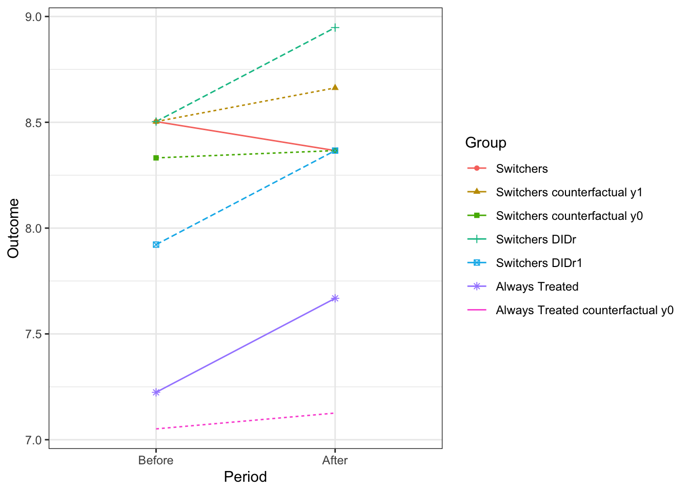

Evolution of average outcomes in the always treated and switchers group in the reverse DID design where everyone is treated in the first period

Figure 4.24: Evolution of average outcomes in the always treated and switchers group in the reverse DID design where everyone is treated in the first period

In Figure 4.24, the effect of the treatment on the switchers is equal to $\hat\Delta^{y_A}_{TUT}=$ 0.3 in the second period and to $\hat\Delta^{y_B}_{TUT}=$ 0.17 in the first period. The $DID$ estimator is equal to $\hat\Delta^{y}_{DID}=$ 0.58 which is of the correct sign but much too big for both treatment effects. The problem is that the change in the outcomes of the always treated (0.44) overestimates the change in outcomes the switchers would have experienced had they stayed in the treatment (0.16). As a consequence, Assumption 4.19 is not valid and the DID estimator is biased. Following Lemma 4.6, the bias of the DID estimator for the effect on the switchers in the second period is equal to the difference in the change of treatment effect over time between always treated ($\hat\Delta^{Y_A}_{TT}-\Delta^{Y_B}_{TT}=$ 0.54 $-$ 0.17 $=$ 0.37) and switchers ($\hat\Delta^{Y_A}_{TUT}-\hat\Delta^{Y_B}_{TUT}=$ 0.3 $-$ 0.17 $=$ 0.12). The bias of the DID estimator for the effect of the treatment on the switchers in the first period is even larger ($\hat B^{y_B}_{DID}=$ 0.41). Following Lemma 4.6, it is close to the change in treatment effect over time among the switchers ($\hat\Delta^{Y_A}_{TT}-\hat\Delta^{Y_B}_{TT}=$ 0.54 $-$ 0.17 $=$ 0.37).

Example 4.41 What happens if we enforce the fact that treatment effects vary in the same way among always takers and switchers. Let’s find out.

param["baralphaAT"] <- 0

Let’s simulate the new data:

set.seed(1234)
N <- 1000
cov.eta.omega <- matrix(c(param["sigma2eta"],0,param["rhoetaomega"]*sqrt(param["sigma2eta"]*param["sigma2omega"]),
                          0,param["sigma2eta"],param["rhoetaomega"]*sqrt(param["sigma2eta"]*param["sigma2omega"]),
                          param["rhoetaomega"]*sqrt(param["sigma2eta"]*param["sigma2omega"]),param["rhoetaomega"]*sqrt(param["sigma2eta"]*param["sigma2omega"]),param["sigma2omega"]),ncol=3,nrow=3,byrow=T)
eta.omega <- as.data.frame(mvrnorm(N,c(0,0,0),cov.eta.omega))
colnames(eta.omega) <- c('etaA','etaB','omega')
mu <- rnorm(N,param["barmu"],sqrt(param["sigma2mu"]))
UB <- rnorm(N,0,sqrt(param["sigma2U"]))
y0B <- mu + UB 
Y0B <- exp(y0B)
Ds <- rep(0,N)
V <- param["gamma"]*(mu-param["barmu"])+eta.omega$omega
Ds[y0B+V<=log(param["barY"])] <- 1 
alphaB <- param["baralphaB"]+  param["thetaB"]*mu + eta.omega$etaB
y1B <- y0B+alphaB
Y1B <- exp(y1B)
epsilonA <- rnorm(N,0,sqrt(param["sigma2epsilon"]))
U0A <- param["rho"]*UB + epsilonA
y0A <- mu +  U0A + param["delta"]
alphaA <- param["baralphaA"]+ param["baralphaAT"]*Ds+ param["thetaA"]*mu + eta.omega$etaA
y1A <- y0A+alphaA
Y0A <- exp(y0A)
Y1A <- exp(y1A)
yA <- y1A*Ds+y0A*(1-Ds)
YA <- Y1A*Ds+Y0A*(1-Ds)
yB <- y1B
YB <- Y1B

Let’s see how DID works on this data.

x <- c("Before","After")
y.AT <- c(mean(yB[Ds==1]),mean(yA[Ds==1]))
y.AT.counterfactual <- c(mean(y0B[Ds==1]),mean(y0A[Ds==1]))
y.Switchers <- c(mean(yB[Ds==0]),mean(yA[Ds==0]))
y.Switchers.counterfactual <- c(mean(y0B[Ds==0]),mean(y0A[Ds==0]))
y.Switchers.counterfactual.1 <- c(mean(y1B[Ds==0]),mean(y1A[Ds==0]))
y.Switchers.DID <- c(mean(yB[Ds==0]),mean(yB[Ds==0])+mean(yA[Ds==1])-mean(yB[Ds==1]))
y.Switchers.DID.1 <- c(mean(yA[Ds==0])-(mean(yA[Ds==1])-mean(yB[Ds==1])),mean(yA[Ds==0]))
data.DID.plot <- as.data.frame(c(y.AT,y.AT.counterfactual,y.Switchers,y.Switchers.counterfactual,y.Switchers.counterfactual.1,y.Switchers.DID,y.Switchers.DID.1))
colnames(data.DID.plot) <- c("Outcome") 
data.DID.plot$Period <- factor(rep(x,7),levels=c("Before","After"))
data.DID.plot$Group <- factor(c("Always Treated","Always Treated","Always Treated counterfactual y0","Always Treated counterfactual y0","Switchers","Switchers","Switchers counterfactual y0","Switchers counterfactual y0","Switchers counterfactual y1","Switchers counterfactual y1","Switchers DIDr","Switchers DIDr","Switchers DIDr1","Switchers DIDr1"),levels=c("Switchers","Switchers counterfactual y1","Switchers counterfactual y0","Switchers DIDr","Switchers DIDr1","Always Treated","Always Treated counterfactual y0"))
data.DID.plot$Observed <- factor(c("Observed","Observed","Unobserved","Unobserved","Observed","Observed","Unobserved","Unobserved","Unobserved","Unobserved","Generated","Generated","Generated","Generated"),levels=c("Observed","Unobserved","Generated"))

WW.before <- (mean(yB[Ds==1])-mean(yB[Ds==0]))
WW.after <- (mean(yA[Ds==1])-mean(yA[Ds==0]))
BA.AT <- mean(yA[Ds==1])-mean(yB[Ds==1])
BA.Switchers <- mean(yA[Ds==0])-mean(yB[Ds==0])
Counterfactual.after <- mean(yB[Ds==0])+BA.AT
DID <- BA.AT  - BA.Switchers
TTASwitchers <- mean(alphaA[Ds==0])
TTBSwitchers <- mean(alphaB[Ds==0])
TTAAT <- mean(alphaA[Ds==1])
TTBAT <- mean(alphaB[Ds==1])

ggplot(data.DID.plot,aes(x=Period,y=Outcome,group=Group,color=Group,shape=Group,linetype=Observed))+
    geom_line() +
    geom_point()+
    scale_linetype_discrete(guide='none') +
    theme_bw()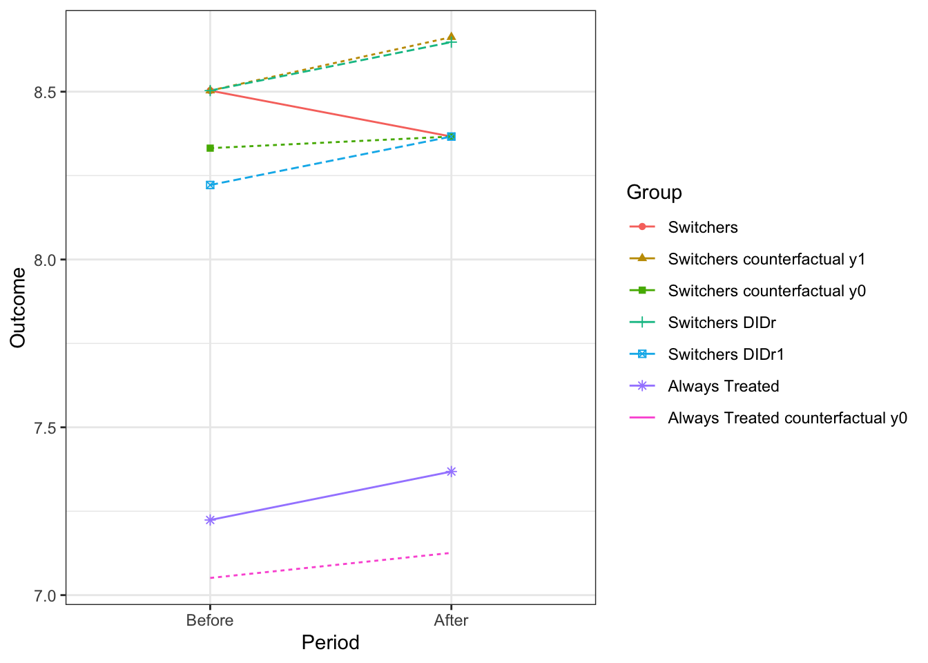

Figure 4.25: Evolution of average outcomes in the always treated and switchers group in the reverse DID design where everyone is treated in the first period and treatment effects that vary in the same way among switchers and always takers

As expected from Theorem 4.16, Figure 4.25 shows that DID almost estimates the effect of the treatment on the switchers in the second period. This makes sense, since the change in outcomes for the switchers in the presence of the treatment (0.16) is well approximated by the observed change in outcomes for the always treated (0.14). According to Lemma 4.6, this is because the change in treatment effect over time for the always treated ($\hat\Delta^{Y_A}_{TT}-\Delta^{Y_B}_{TT}=$ 0.24 $-$ 0.17 $=$ 0.07) is close to the change in treatment effect over time for the switchers ($\hat\Delta^{Y_A}_{TUT}-\hat\Delta^{Y_B}_{TUT}=$ 0.3 $-$ 0.17 $=$ 0.12). Note that the DID estimator is still biased for the effect of the treatment on the switchers in the first period, because the treatment effect on the always takers changes over time (Lemma 4.6).

Remark. Note that in this model, DID does not identify $\Delta^{Y_A}_{TUT}$. The reasons why are left as an exercise.

Remark. We can relax Assumption 4.22 by redefining the potential outcomes observed after the switchers exit from the treatment as the potential outcomes observed when the treatment stops after having been experienced. One way to parameterize this potential outcome is to make it a function of the time elapsed since exiting the treatment: $Y^0_{i,t}(\tau)$, where $\tau$ denotes the number of periods after exiting the treatment. For the switchers, in period $A$, $\tau=1$, for example. One can then show that the DID estimator identifies the effect of the treatment relative to exiting the treatment: $\Delta^Y_{DID}=\esp{Y^1_{i,A}-Y^0_{i,A}(1)|D_i=0}$ under Assumptions 4.21 and 4.19. The proof is left as an exercise.

4.3.3 Difference In Differences with multiple time periods

In real life, we generally have access to several time periods before and after the treatment date. What happens to DID in that case? Well, several things actually happen:

We now have several pre-treatment observations for each unit. Which one should we choose to form our DID estimator? If we use all of them, should we combine them? If yes, how?
We also have several post-treatment observations. Which one should we choose to form our DID estimator? If we use all of them, should we combine them? If yes, how?
We also have some units that will be treated for several periods in a row. Should we use them to form a $DID^r$ estimator? If yes, should we combine them with the DID estimates? If yes, how?
We also might have some units that exit the treatment after some time. Should we use them to form a DID estimator? Should we combine this estimate with the others? If yes, how?

There is a lot of questions. In order to be able to answer them, I am for the moment going to abstract from the last one. I am going to assume that once a unit has entered the treatment, it cannot exit it. DID designs such as these are called staggered designs. This is obviously a very strong assumption, but we will relax it at some point. Let’s go now.

4.3.3.1 Identification

In this section, we are going to define rigorously the setting that we have in front of us and the several treatment effects that we might want to estimate. This will be the most important part of the identification exercise. Once the definitions are in place, identification will be mostly straightforward.

In a DID design with multiple time periods, time flows from $t=1$ to $t=T$. $D_{i,t}$ takes value one when unit $i$ is treated at period $t$ and zero otherwise. In a staggered design, once treated, a unit is treated forever (the treatment is said to be an absorbing state). As a consequence, we can characterize units by the date at which they start to be treated. We are going to call this variable $D_{i}$ and it takes values in the set $\left\{1,2,\dots,T,\infty\right\}$. Units treated at period $1$ (or even before, we cannot say for sure) are always treated in a staggered design. Then, units enter at successive periods until the last one. Finally, some units may never receive the treatment (never takers). By convention, we denote them with $D_{i}=\infty$.

We can define a separate treatment effect for each of the treatment groups and for each time period: $\Delta^{Y_{\tau}}_{TT_d}=\esp{Y^1_{i,d+\tau}-Y^0_{i,d+\tau}|D_i=d}$, for $\tau,d\in\left\{1,2,\dots,T\right\}$.

We can also form a very large bunch of DID estimators:

\[\begin{align*} \Delta^{Y}_{DID}(d,d',\tau,\tau') & = \esp{Y_{i,d+\tau}|D_i=d}-\esp{Y_{i,d-\tau'}|D_i=d}-(\esp{Y_{i,d+\tau}|D_i=d'}-\esp{Y_{i,d-\tau'}|D_i=d'}), \end{align*}\]

where $\tau,\tau'>0$ and $d'>d+\tau$. $\Delta^{Y}_{DID}(d,d',\tau,\tau')$ tries to estimate the effect of the treatment on units that first entered the treatment at period $t=d$ (the treated group here) using the units that received the treatment at period $d'>d$ as a benchmark. $\Delta^{Y}_{DID}(d,d',\tau,\tau')$ compares how outcomes have changed between $\tau$ periods after the treatment and $\tau'$ periods before the treatment.

Imposing $d'>d+\tau$ ensures that $\Delta^{Y}_{DID}(d,d',\tau,\tau')$ is a proper DID estimator. If $d-\tau'<d'<d+\tau$, $\Delta^{Y}_{DID}(d,d',\tau,\tau')$ is not a proper DID estimator since units in group $d'$ also receive the treatment between the two dates at which outcomes are measured. When $d'<d-\tau'$, $\Delta^{Y}_{DID}(d,d',\tau,\tau')$ compares the change in outcomes in the group entering the treatment at date $d$ with the changes in outcomes occurring in a group that has already entered the treatment at a date $d'$ that is prior the starting date of the DID. Since this estimator is a $DID^r$ estimator, I am going to denote it as such in the future. $\Delta^{Y}_{DID^r}(d,d',\tau,\tau')$ is well-defined only when $d'<d-\tau'$.

Before stating our first identification result, let us make some assumptions that will mirror the simpler ones we made in the previous section. First, we are going to assume that at least some units are untreated at some period:

Hypothesis 4.23 (Some Units are Not Treated) We assume that not all units in the population are treated in the first period: $\Pr(D_i=1)<1$.

Next, we assume that agents cannot anticipate the treatment:

Hypothesis 4.24 (No Anticipation Effects over Time) We assume that agents cannot anticipate that the program will happen and that they do not change their behavior as a consequence: $Y_{i,t}=Y^0_{i,t}$, $\forall i\in \left\{i:D_i=d\right\}$, $\forall t<d$.

As a consequence of Assumptions 4.23 and 4.24, we can write observed outcomes as a function of treatment and potential outcomes using the usual switching equation.

The final very important assumption that we can make is to assume that the trends in the potential outcomes in the absence the treatment are the same for the treated and the untreated units:

Hypothesis 4.25 (Parallel Trends for All Groups) We assume that the trends in the potential outcomes in the absence the treatment are the same for all the treatment groups:

\[\begin{align*} \forall d,t,t'\in\left\{1,2,\dots,T\right\}, & \esp{Y^0_{i,t}|D_i=d} - \esp{Y^0_{i,t'}|D_i=d} = \esp{Y^0_{i,t}|D_i=\infty} - \esp{Y^0_{i,t'}|D_i=\infty}. \end{align*}\]

We are now ready to state our main identification result:

Theorem 4.18 (DID identifies TT at Each Point in Time) Under Assumptions 4.23, 4.24 and 4.25, the DID estimator identifies the average effect of the Treatment on the Treated in each time period:

\[\begin{align*} \Delta^{Y}_{DID}(d,d',\tau,\tau') & = \Delta^{Y_{\tau}}_{TT_d}, \end{align*}\] where $\tau,\tau'>0$ and $d'>d+\tau$.

Proof. \[\begin{align*} \Delta^{Y}_{DID}(d,d',\tau,\tau') & = \esp{Y_{i,d+\tau}-Y_{i,d-\tau'}|D_i=d}-\esp{Y_{i,d+\tau}-Y_{i,d-\tau'}|D_i=d'}\\ & = \esp{Y^1_{i,d+\tau}-Y^0_{i,d-\tau'}|D_i=d}-\esp{Y^0_{i,d+\tau}-Y^0_{i,d-\tau'}|D_i=d'}\\ & = \esp{Y^1_{i,d+\tau}-Y^0_{i,d-\tau'}|D_i=d}-\esp{Y^0_{i,d+\tau}-Y^0_{i,d-\tau'}|D_i=d}\\ & = \esp{Y^1_{i,d+\tau}-Y^0_{i,d+\tau}|D_i=d} \end{align*}\]

where the second equality follows from Assumptions 4.23 and 4.24 and the fact that $d'>d+\tau$. The third equality follows from Assumption 4.25. This proves the result.

Theorem 4.18 shows that the basic mechanics of the DID estimator extends to multiple periods. The problem with Theorem 4.18 is that we now have multiple ATT estimates for various groups and time periods, using various time periods and groups as reference. How do we reconcile all of these estimates in a unique parameter, or at least a vector of parameters that makes some sense? Let’s define sets of positive weights $w^k(d,d',\tau,\tau')$ that sum to one. We can then define a set of DID estimators:

\[\begin{align*} \Delta^{Y}_{DID}(k)=\sum w^k(d,d',\tau,\tau')\Delta^{Y}_{DID}(d,d',\tau,\tau'), \end{align*}\]

where the sum is taken in coherence with the weights. These DID estimators are going to identify various features of the effects of the treatment, using various types of reference groups and time periods. Let us be more precise:

A first set of weights combines the various estimates of the same treatment effect on the outcomes of group $d$ observed at period $d=\tau$. These weights, which we denote $w^s_{d,\tau}(d',\tau')$, are such that they take value zero for estimates $\Delta^{Y}_{DID}(d'',d',\tau'',\tau')$ that are such $d''\neq d$ and $\tau''\neq\tau$ and they have: $\sum_{\tau',d'>d+\tau}w^s_{d,\tau}(d',\tau')=1$. One way to define these weights is to make them proportional to the proportion of $(d',\tau')$ groups of observations in the population.
A second set of weights is going to combine the treatment effects themselves. For example, one might want to measure the average effect of the treatment $\tau$ periods after entering it. This type of dynamic treatment effect is useful to measure how the effect of the treatment varies over time. There are two versions of this set of weights: one unconditional and one conditional on at least reaching a certain number of periods in the treatment (let’s say $\tau''>\tau$ periods after the treatment). With the second version, all the estimates of the dynamic effects of the treatment are going to be taken over the same set of groups. With the first version, changes in treatment effects over time might be confounded by changes in group composition. Let’s denote the first type of weights $w^u_{\tau}(d,d',\tau')$ and the second $w^c_{\tau,\tau''}(d,d',\tau')$ , with $\tau''>\tau$. We then have $\Delta^{Y_u}_{DID}(\tau)=\sum_{d,d'>d+\tau,\tau'} w^u_{\tau}(d,d',\tau')\Delta^{Y}_{DID}(d,d',\tau,\tau')$ and $\Delta^{Y_c}_{DID}(\tau,\tau'')=\sum_{d,d'>d+\tau,\tau'} w^c_{\tau,\tau''}(d,d',\tau')\Delta^{Y}_{DID}(d,d',\tau,\tau')$. These effects can also be restricted to versions using a single reference period $\tau'$ to build the DID estimator: $\Delta^{Y_u}_{DID}(\tau,\tau')$ and $\Delta^{Y_c}_{DID}(\tau,\tau',\tau'')$.
A third set of effects is simply taking the average of all the treatment effects at a given time period. Let’s denote these set of weights $w^t(d,d',\tau,\tau')$ for the effect observed at period $t$. Then, we have $\Delta^{Y_t}_{DID}=\sum_{\tau+d=t,d'>d+\tau,\tau'} w^t(d,d',\tau,\tau')\Delta^{Y}_{DID}(d,d',\tau,\tau')$. Another version again uses only estimates taken with period $d-\tau'$ as a reference: $\Delta^{Y_t}_{DID}(\tau')=\sum_{\tau+d=t,d'>d+\tau} w^t_{\tau'}(d,d',\tau)\Delta^{Y}_{DID}(d,d',\tau,\tau')$.
Finally, one can simply define the overall effect of the treatment on the treated as the sum of all relevant treatment effects estimated in the sample. Let’s define the set of weights $w^a(d,d',\tau,\tau')$ and the estimate of the average treatment effect on the treated as $\Delta^{Y}_{DID}=\sum_{\tau,d,d'>d+\tau,\tau'} w^a(d,d',\tau,\tau')\Delta^{Y}_{DID}(d,d',\tau,\tau')$. Again, some authors restrict this estimate to be specific to a given reference period: $\Delta^{Y}_{DID}(\tau')=\sum_{\tau,d,d'>d+\tau} w^a_{\tau'}(d,d',\tau)\Delta^{Y}_{DID}(d,d',\tau,\tau')$.

As a consequence of Theorem 4.18, all the aggregate treatment effects are identified, as long as each of their separate components are identified. The following corollary makes that clear:

Corollary 4.3 (DID identifies Weighted TT) Under Assumptions 4.23, 4.24 and 4.25, assuming that $\Pr(D_i=d)>0$ and $\Pr(D_i=d')>0$, $\forall (d,d')\in \left\{1,2,\dots,T,\infty\right\}$ such that $w^k(d,d',\tau,\tau')>0$ and assuming that $\forall d,d',\tau,\tau'$ such that $w^k(d,d',\tau,\tau')>0$, $(d+\tau,d'-\tau')\in\left\{1,2,\dots,T,\infty\right\}^2$, the weighted DID estimator identifies the corresponding weigthed average of Treatment on the Treated:

\[\begin{align*} \Delta^{Y}_{DID}(k) & = \Delta^{Y}_{TT}(k), \end{align*}\] with \[\begin{align*} \Delta^{Y}_{TT}(k) & = \sum w^k(d,d',\tau,\tau')\Delta^{Y_{\tau}}_{TT_d} \end{align*}\]

Proof. The proof follows from Theorem 4.18: as long as the groups for which the weights are non null exist, and the time periods for which the weights are non null also exist in the data, Theorem 4.18 ensures that each of the components of the weighted average is identifed and thus the weighted average is identified as well.

Before going through an example to illustrate all of these notions, let me introduce one estimator.

4.3.3.2 Estimation

Estimation of the various DID estimators that we have defined in the previous section can take several forms. The simplest form estimates the separate individual DID components using the methods seen in Section 4.3.1, and then manually computes their weighted averages. I will detail this approach first. A very similar approach uses the estimates obtained with one reference period (in general $\tau'=1$) and combines them to obtain one treatment effect or a series of treatment effects around the treatment date. This approach has been proposed by Sun and Abraham (2021) and by Callaway and Sant’Anna (2021). A more intricate approach uses an imputation model to derive the predicted counterfactual values for all treated observations and then averages them. This approach has been proposed by Borusyak, Jaravel and Speiss (2021), Liu, Wang and Xu (2021) and Gardner (2021). de Chaisemartin and d’Haultfoeuille (2020) propose to only use changes that occur around the treatment date. Finally, one could use the Two Way Fixed Effects model presented in Section 4.3.1, combining all the time periods in a single estimator. Recent work by Goodman-Bacon (2021) has shown that this approach is only valid under much more restrictive assumptions than the ones stated in Corollary 4.3. The main reason for why it is so is that the Two Way Fixed Effects estimator combines individual DID and $DID^r$ estimates, thereby generating strong biases if the assumptions that ensure the validity of $DID^r$ are not valid. An extension to the Two Way Fixed Effects estimator, the stacked DID estimator, restores its good properties. It has been proposed by Cengiz, Dube, Lindner and Zipperer (2019) and extended by Gardner (2021). The R packages required to implement all of these estimators are listed on Asjad Naqvi’s DID webpage. We are going to see how they perform on our data.

4.3.3.2.1 Using weighted averages of individual DID estimators

This estimator is pretty simple to define. Simply take all the possible $2\times2$ possible DID estimators $\Delta^{Y}_{DID}(d,d',\tau,\tau')$, with $\tau,\tau'>0$ and $d'>d+\tau$, and then average them using the pre-defined weights $w^k(d,d',\tau,\tau')$ of your choice. The key to this section is to illustrate how to operationalize this approach in practice with an example. Let’s go.

Example 4.42 The key here is first to generate some data.

We are going to have four successive time periods, $1$, $2$, $3$, and $4$. At each of these time periods, some units start receiving the treatment, generating four treatment groups: $D_i\in\{1,2,3,4\}$. Let us write a model compatible with this setting, choose a parameterization and generate the data.

\[\begin{align*} y^1_{i,t} & = y_{i,t}^0+\bar{\alpha}_t+\sum_{d}(\bar{\alpha}_{t,d}+\theta_d\mu_i)\uns{D_{i,d}=1}+\eta_{i,t} \\ y^0_{i,t} & = \mu_i+\delta_t+U^0_{i,t} \\ U^0_{i,t} & = \rho U^0_{i,t-1}+\epsilon_{i,t} \\ D_{i,t} & = \uns{y^0_{i,1} + \xi_t+ V_i\leq\bar{y}} \\ V_i & = \gamma(\mu_i-\bar{\mu}) + \omega_{i,1} \\ U^0_{i,1} & \sim\mathcal{N}(0,\sigma^2_{U}) \\ \mu_i & \sim\mathcal{N}(\bar{\mu},\sigma^2_{\mu}) \\ (\eta_{i,t},\omega_{i,t}) & \sim\mathcal{N}(0,0,\sigma^2_{\eta},\sigma^2_{\omega},\rho_{\eta,\omega})\\ \epsilon_{i,t} & \sim\mathcal{N}(0,\sigma^2_{\epsilon}). \end{align*}\]

I am going to parameterize the $\bar{\alpha}_{t,d}$ process in order to avoid having to specify the 14 parameters that it otherwise would require. The parameterization I am choosing is $\bar{\alpha}_{t,d}=\bar\chi_d+\kappa_d(t-d)\uns{t\geq d}$, so that treatment effects increase linearly as time into the treatment increases. Let us now choose some parameter values:

param <- c(8,.5,.28,1500,0.9,
           0.01,0.01,0.01,0.01,
           0.05,0.05,
           0,0.1,0.2,0.3,
           0.05,0.1,0.15,0.2,
           0.25,0.1,0.05,0,
           1.5,1.25,1,0.75,
           0.5,0,-0.5,-1,
           0.1,0.28,0)
names(param) <- c("barmu","sigma2mu","sigma2U","barY","rho",
                  "theta1","theta2","theta3","theta4",
                  "sigma2epsilon","sigma2eta",
                  "delta1","delta2","delta3","delta4",
                  "baralpha1","baralpha2","baralpha3","baralpha4",
                  "barchi1","barchi2","barchi3","barchi4",
                  "kappa1","kappa2","kappa3","kappa4",
                  "xi1","xi2","xi3","xi4",
                  "gamma","sigma2omega","rhoetaomega")

Let us now generate the corresponding data (in long format):

set.seed(1234)
N <- 1000
T <- 4
cov.eta.omega <- matrix(c(param["sigma2eta"],param["rhoetaomega"]*sqrt(param["sigma2eta"]*param["sigma2omega"]),param["rhoetaomega"]*sqrt(param["sigma2eta"]*param["sigma2omega"]),param["sigma2omega"]),ncol=2,nrow=2)
data <- as.data.frame(mvrnorm(N*T,c(0,0),cov.eta.omega))
colnames(data) <- c('eta','omega')
# time and individual identifiers
data$time <- c(rep(1,N),rep(2,N),rep(3,N),rep(4,N))
data$id <- rep((1:N),T)
# unit fixed effects
data$mu <- rep(rnorm(N,param["barmu"],sqrt(param["sigma2mu"])),T)
# time fixed effects
data$delta <- c(rep(param["delta1"],N),rep(param["delta2"],N),rep(param["delta3"],N),rep(param["delta4"],N))
data$baralphat <- c(rep(param["baralpha1"],N),rep(param["baralpha2"],N),rep(param["baralpha3"],N),rep(param["baralpha4"],N))

# building autocorrelated error terms
data$epsilon <- rnorm(N*T,0,sqrt(param["sigma2epsilon"]))
data$U[1:N] <- rnorm(N,0,sqrt(param["sigma2U"]))
data$U[(N+1):(2*N)] <- param["rho"]*data$U[1:N] + data$epsilon[(N+1):(2*N)]
data$U[(2*N+1):(3*N)] <- param["rho"]*data$U[(N+1):(2*N)] + data$epsilon[(2*N+1):(3*N)]
data$U[(3*N+1):(T*N)] <- param["rho"]*data$U[(2*N+1):(3*N)] + data$epsilon[(3*N+1):(T*N)]
# potential outcomes in the absence of the treatment
data$y0 <- data$mu + data$delta + data$U 
data$Y0 <- exp(data$y0)
# treatment timing
# error term
data$V <- param["gamma"]*(data$mu-param["barmu"])+data$omega
# treatment group, with 99 for the never treated instead of infinity
Ds <- if_else(data$y0[1:N]+param["xi1"]+data$V[1:N]<=log(param["barY"]),1,
              if_else(data$y0[1:N]+param["xi2"]+data$V[1:N]<=log(param["barY"]),2,
                      if_else(data$y0[1:N]+param["xi3"]+data$V[1:N]<=log(param["barY"]),3,
                              if_else(data$y0[1:N]+param["xi4"]+data$V[1:N]<=log(param["barY"]),4,99))))
data$Ds <- rep(Ds,T)
# Treatment status
data$D <- if_else(data$Ds>data$time,0,1)
# potential outcomes with the treatment
# effect of the treatment by group
data$baralphatd <- if_else(data$Ds==1,param["barchi1"],
                           if_else(data$Ds==2,param["barchi2"],
                                   if_else(data$Ds==3,param["barchi3"],
                                           if_else(data$Ds==4,param["barchi4"],0))))+
                  if_else(data$Ds==1,param["kappa1"],
                           if_else(data$Ds==2,param["kappa2"],
                                   if_else(data$Ds==3,param["kappa3"],
                                           if_else(data$Ds==4,param["kappa4"],0))))*(data$time-data$Ds)*if_else(data$time>=data$Ds,1,0)
data$y1 <- data$y0 + data$baralphat + data$baralphatd + if_else(data$Ds==1,param["theta1"],if_else(data$Ds==2,param["theta2"],if_else(data$Ds==3,param["theta3"],param["theta4"])))*data$mu + data$eta
data$Y1 <- exp(data$y1)
data$y <- data$y1*data$D+data$y0*(1-data$D)
data$Y <- data$Y1*data$D+data$Y0*(1-data$D)

Let us now plot the data, especially the potential outcomes for each group.

dataplotDIDStaggered <- data %>%
                          group_by(Ds,time) %>%
                          summarize(
                            y1=mean(y1),
                            y0=mean(y0)
                          ) %>%
                          pivot_longer(cols=c("y1","y0"),values_to="Outcome",names_to="PotentialOutcome") %>%
                          mutate(
                            TreatmentDate = factor(Ds,levels=c("99","4","3","2","1"))
                          )

ggplot(dataplotDIDStaggered,aes(x=time,y=Outcome,color=TreatmentDate,shape=TreatmentDate,linetype=PotentialOutcome))+
      geom_line() +
      geom_point()+
#    scale_linetype_discrete(guide='none') +
    theme_bw()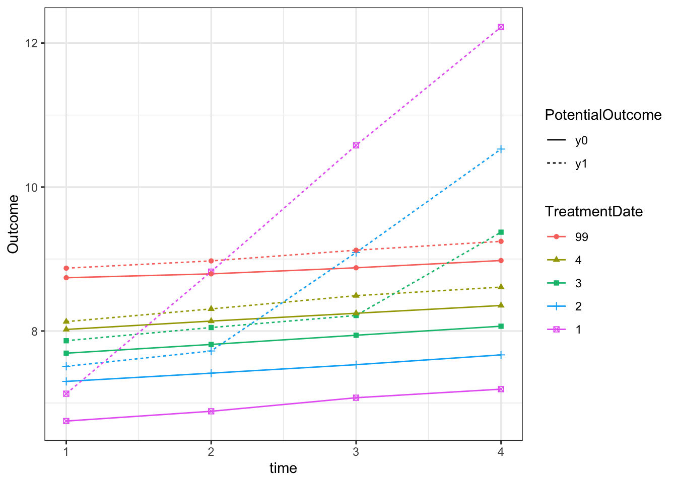

Figure 4.26: Evolution of average outcomes in the various treatment groups defined by their date of entry into the treatment

Figure 4.26 shows that the first units to be treated have the lowest potential outcomes in the absence of the treatment ($y^0$, in full line), and that each successive cohort entering the treatment over time has increasingly large potential outcomes. Assumption 4.25 seems to hold in this dataset, at least visually: the trends in potential outcomes in the absence of the treatment seem to be rather parallel to each other in each group. Once a group of unit has entered the treatment, it experiences an increase in outcomes that grows over time. Finally, note that we will be unable to estimate the impact on the group with $D_i=1$ since they enter the treatment at the first period.

Let us now compute each possible DID estimator on this dataset. In order to save some space and time, we will start by focusing on group 2. Group 2 starts treatment at period 2, and thus only period 1 can be used for building a DID estimator. But several comparison groups exist: the never treated (note that we have used $D_i=99$ instead of $D_i=\infty$ to characterize this group, in order to make it simpler to manipulate it in R) but also group 3, that can serve as an untreated benchmark between periods 1 and 2, and group 4, which can be used as an untreated benchmark in periods 1, 2 and 3. Let’s compute all these effects. In order to make our lives simpler, we are going to generate a function to generate $\hat\Delta^{Y}_{DID}(d,d',\tau,\tau')$.

# StaggeredDID22 is a function that takes as inputs:
# y: name of outcome variable (character)
# D: name of treatment group variable (character)
# d: treatment group defined by date of entry into the treatment
# dprime: comparison group
# tau: number of periods after treatment date at which we estimate the effect of the treatment
# tauprime: number of periods before the treatment date that we use a baseline period (defaults to one)
# t: time indicator (character)
# i: individual unit indicator (character)
# data: dataset containing the outcomes and treatments and time and unit indicators
StaggeredDID22 <- function(tau,y,D,d,dprime,tauprime=1,t,i,data){
  # taking out the irrelevant groups and time periods and generating a useful treatment variable
  data.DID <- data %>%
            filter(!!sym(D)==d | !!sym(D)==dprime) %>% 
            filter(time==d+tau | time==d-tauprime) %>%
            mutate(
              Dit = if_else(!!sym(D)==d & time==d+tau,1,0)
            )
  # running the within estimator (fixest)
  # regression formula
  DID.form <- as.formula(paste(paste(y,paste("Dit",t,sep="+"),sep="~"),i,sep="|"))
  reg.W.fixest <- feols(DID.form, data = data.DID)
  # result vector
  DID.est.W.fixest <- c(d,dprime,tau,tauprime,coef(reg.W.fixest)[[1]],sqrt(vcov(reg.W.fixest)[[1,1]]))
  names(DID.est.W.fixest) <- c("d","dprime","tau","tauprime","DIDest","DIDse")
  return(DID.est.W.fixest)
}

# Run the regression and keep results
# D=99 as benchmark
# list of tau for d=2 and dprime=99 and tauprime=1
tau.2.99 <- c(0,1,2)
DID.2.99.1 <- map_dfr(tau.2.99,StaggeredDID22,y='y',D='Ds',d=2,dprime=99,tauprime=1,t="time",i="id",data=data) 
# D=3 
# list of tau for d=2 and dprime=3 and tauprime=1
tau.2.3 <- c(0)
DID.2.3.1 <- map_dfr(tau.2.3,StaggeredDID22,y='y',D='Ds',d=2,dprime=3,tauprime=1,t="time",i="id",data=data) 
# D=4 
# list of tau for d=2 and dprime=4 and tauprime=1
tau.2.4 <- c(0,1)
DID.2.4.1 <- map_dfr(tau.2.4,StaggeredDID22,y='y',D='Ds',d=2,dprime=4,tauprime=1,t="time",i="id",data=data) 

# regroup results
DID.2.1 <- rbind(DID.2.99.1,DID.2.3.1,DID.2.4.1)

# true effects (in the sample)
ATT.2.0 <- mean(data$y1[data$Ds==2 & data$time==2])-mean(data$y0[data$Ds==2 & data$time==2])
ATT.2.1 <- mean(data$y1[data$Ds==2 & data$time==3])-mean(data$y0[data$Ds==2 & data$time==3])
ATT.2.2 <- mean(data$y1[data$Ds==2 & data$time==4])-mean(data$y0[data$Ds==2 & data$time==4])

Let us now plot the results for the DID estimates on group $2$ using $\tau'=1$ as a benchmark pre-treatment period.

# preparing data
DID.2.1 <- DID.2.1 %>%
            mutate(
              dprime=factor(dprime,levels=c("99","4","3","2","1"))
            )

# plot
ggplot(DID.2.1,aes(x=tau,y=DIDest,colour=dprime,linetype=dprime))+
      geom_line() +
    geom_pointrange(aes(ymin=DIDest-1.96*DIDse,ymax=DIDest+1.96*DIDse))+
    ylab("DID estimate") +
    xlab("Time after treatment (tau)") +
    scale_x_continuous(breaks=c(0,1,2)) +
    expand_limits(y=0) +
    scale_colour_discrete(name="Comparison\ngroup")+
    scale_linetype_discrete(name="Comparison\ngroup")+
    theme_bw()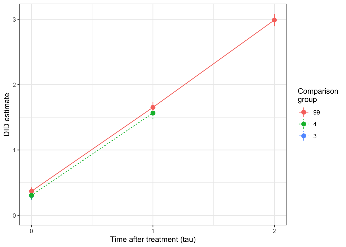

$DID estimates for Group 2 at various time periods after the treament and with various comparison groups and with the reference period $\tau'=1$$

Figure 4.27: DID estimates for Group 2 at various time periods after the treament and with various comparison groups and with the reference period $\tau'=1$

Figure 4.27 shows the $\hat\Delta^{Y}_{DID}(d,d',\tau,\tau')$ estimates for $d=2$ and $\tau'=1$, varying both $\tau$ and $d'$. The treatment effects estimated using different reference groups are similar to each other when we can compare them. Moreover, the treatment effect grows with time, as expected from Figure 4.26. The true effects of the treatment on group 2 are, in our sample: $\hat\Delta^{Y_{0}}_{TT_2}=$ 0.31, $\hat\Delta^{Y_{1}}_{TT_2}=$ 1.56 and $\hat\Delta^{Y_{2}}_{TT_2}=$ 2.86. These are very close to our DID estimates. For example, $\hat\Delta^{Y}_{DID}(2,99,0,1)=$ 0.37, while $\hat\Delta^{Y}_{DID}(2,4,0,1)=$ 0.31 and $\hat\Delta^{Y}_{DID}(2,3,0,1)=$ 0.3, which are all pretty close to $\hat\Delta^{Y_{0}}_{TT_2}=$ 0.31. $\hat\Delta^{Y}_{DID}(2,99,1,1)=$ 1.65, while $\hat\Delta^{Y}_{DID}(2,4,1,1)=$ 1.57, which are also all pretty close to $\hat\Delta^{Y_{1}}_{TT_2}=$ 1.56. Finally, $\hat\Delta^{Y}_{DID}(2,99,2,1)=$ 2.99, while $\hat\Delta^{Y_{2}}_{TT_2}=$ 2.86.

In order to aggregate the estimates presented in Figure 4.27, we could for example use the proportion of each comparison group in the sample and average the treatment effects for each post treatment period $\tau$ with these weights. We can do the same thing with groups 3 and 4 and see what happens. Note that with these two groups, I can also estimate a placebo test: that is the effect of the treatment before the treatment takes place. Such event study estimates have become standard in the DID literature. I will expand on these tests in Section ??. For group 3, I can estimate the effect for $\tau\in\{-2,0,1\}$ and for group 4, for $\tau\in\{-3,-2,0\}$, when the benchmark group is the never treated group.

# do the DID22 estimates for d=3
# Run the regression and keep results
# D=99 as benchmark
# list of tau for d=3 and dprime=99 and tauprime=1
tau.3.99 <- c(-2,0,1)
DID.3.99.1 <- map_dfr(tau.3.99,StaggeredDID22,y='y',D='Ds',d=3,dprime=99,tauprime=1,t="time",i="id",data=data) 
# D=4 as a benchmark 
# list of tau for d=3 and dprime=4 and tauprime=1
tau.3.4 <- c(-2,0)
DID.3.4.1 <- map_dfr(tau.3.4,StaggeredDID22,y='y',D='Ds',d=3,dprime=4,tauprime=1,t="time",i="id",data=data) 

# regroup results
DID.3.1 <- rbind(DID.3.99.1,DID.3.4.1)

# true effects (in the sample)
ATT.3.0 <- mean(data$y1[data$Ds==3 & data$time==3])-mean(data$y0[data$Ds==3 & data$time==3])
ATT.3.1 <- mean(data$y1[data$Ds==3 & data$time==4])-mean(data$y0[data$Ds==3 & data$time==4])

# do the DID22 estimates for d=4
# Run the regression and keep results
# D=99 as benchmark
# list of tau for d=4 and dprime=99 and tauprime=1
tau.4.99 <- c(-3,-2,0)
DID.4.99.1 <- map_dfr(tau.4.99,StaggeredDID22,y='y',D='Ds',d=4,dprime=99,tauprime=1,t="time",i="id",data=data) 

# true effects (in the sample)
ATT.4.0 <- mean(data$y1[data$Ds==4 & data$time==4])-mean(data$y0[data$Ds==4 & data$time==4])

# regrouping all effects
DID.1 <- rbind(DID.2.1,DID.3.1,DID.4.99.1)

# computing the weights
prop.groups.DID <- data %>%
                    filter(time==1) %>%
                    group_by(Ds) %>%
                    summarize(
                      prop.group = n()/N
                    ) %>%
                    rename(
                      dprime=Ds
                    )%>%
                    mutate(
                      dprime=factor(dprime,levels=c("99","4","3","2","1"))
                    )

# joining the weights to the results
DID.1 <- DID.1 %>%
          left_join(prop.groups.DID,by=c("dprime"))

# generating the weighted averages by tau 
DID.tau <- DID.1 %>%
            mutate(
              w.ATT = prop.group*DIDest
            ) %>%
            group_by(tau,d) %>%
            summarize(
              sum.w.ATT = sum(w.ATT),
              sum.w = sum(prop.group)
            ) %>% 
            mutate(
              ATT.tau = sum.w.ATT/sum.w
            ) %>%
            select(d,tau,ATT.tau) %>%
            mutate(
              d=factor(d,levels=c("2","3","4"))
            ) 

# adding the reference period
DID.ref <- as.data.frame(rbind(c(2,-1,0),c(3,-1,0),c(4,-1,0)))
colnames(DID.ref) <- colnames(DID.tau)
DID.ref$d <- factor(DID.ref$d,levels=c("2","3","4"))

DID.tau <- rbind(DID.tau,DID.ref)

Let us now plot the results for the DID estimates in groups $2$, $3$ and $4$ using $\tau'=1$ as a benchmark pre-treatment period and aggregating the estimates using every possible valid control group:

ggplot(DID.tau,aes(x=tau,y=ATT.tau,colour=d,linetype=d))+
    geom_line() +
    geom_point() +
    ylab("DID estimate") +
    xlab("Time after treatment (tau)") +
    scale_x_continuous(breaks=c(-3,-2,-1,0,1,2)) +
    expand_limits(y=0) +
    scale_colour_discrete(name="Treatment\ngroup")+
    scale_linetype_discrete(name="Treatment\ngroup")+
    theme_bw()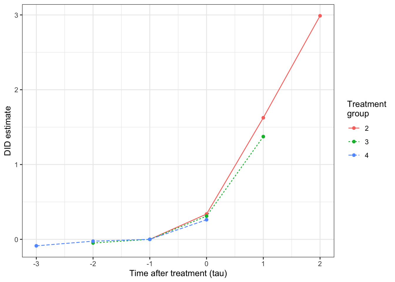

$DID estimates for all groups at various time periods after the treament aggregated across all comparison groups and with the reference period $\tau'=1$$

Figure 4.28: DID estimates for all groups at various time periods after the treament aggregated across all comparison groups and with the reference period $\tau'=1$

On Figure 4.28, we can see that all the estimators are comparable for each other at each time period $\tau$, no matter the treatment group. We thus can aggregate the impacts at each period $\tau$ across all treatment groups. There are two ways to do that: one is to use all the groups for which we observe the effect of the treatment at period $\tau$. The drawback of this approach is that group composition changes with $\tau$. For example, on Figure 4.28, we can see that the treatment group treated in the last period (for which $D_i=4$) contributes only to the computation of the effect of the treatment at period $\tau=0$. This is because we cannot observe what happens to this group in later periods with our dataset. As a consequence, in period $\tau=0$, all three groups–$D_i=2$, $D_i=3$ and $D_i=4$–contribute to the estimation of the effect of the treatment, whereas only groups with $D_i=2$ and $D_i=3$ contribute to the estimation of the effect at $\tau=1$, and only $D_i=2$ contributes to estimating the effect at $\tau=2$. If treatment effects were heterogeneous across treatment groups, this change in group composition would confound actual changes in the magnitude of treatment effects. Since the effect of the treatment is rather homogenous across groups, this group comopsition problem will not matter in our application. Nevertheless, we are still going to estimate the effect of the treatment at $\tau=0$ and $\tau=1$ maintaining group composition constant ($D_i=2$ and $D_i=3$). In our application, both approaches will yield very similar results. The weights we are going to use for our aggregation are the proportions of units belonging to each group.

# joining the weights to the results
DID.tau <- DID.tau %>%
          left_join(prop.groups.DID,by=c("d"="dprime"))

# generating the weighted averages by tau (varying group composition)
DID.tau.agg <- DID.tau %>%
            mutate(
              w.ATT = prop.group*ATT.tau
            ) %>%
            group_by(tau) %>%
            summarize(
              sum.w.ATT = sum(w.ATT),
              sum.w = sum(prop.group)
            ) %>% 
            mutate(
              ATT.tau.agg = sum.w.ATT/sum.w
            ) %>%
            select(tau,ATT.tau.agg) %>%
            mutate(
              Composition="Varying"
            )

# generating the weighted averages by tau (constant group composition)
DID.tau.agg.cst <- DID.tau %>%
            filter(d==2 | d==3) %>%
            filter(tau==0 | tau==1) %>%
            mutate(
              w.ATT = prop.group*ATT.tau
            ) %>%
            group_by(tau) %>%
            summarize(
              sum.w.ATT = sum(w.ATT),
              sum.w = sum(prop.group)
            ) %>% 
            mutate(
              ATT.tau.agg = sum.w.ATT/sum.w
            ) %>%
            select(tau,ATT.tau.agg) %>%
            mutate(
              Composition="Constant"
            )

#regrouping estimates
DID.tau.agg.tot <- rbind(DID.tau.agg,DID.tau.agg.cst) %>%
                    mutate(
                      Composition = factor(Composition,levels=c("Constant","Varying"))
                    )

Let’s plot the resulting estimates.

ggplot(DID.tau.agg.tot,aes(x=tau,y=ATT.tau.agg,colour=Composition,linetype=Composition))+
    geom_line() +
    geom_point() +
    ylab("DID estimate") +
    xlab("Time after treatment (tau)") +
    scale_x_continuous(breaks=c(-3,-2,-1,0,1,2)) +
    expand_limits(y=0) +
    scale_colour_discrete(name="Group\ncomposition")+
    scale_linetype_discrete(name="Group\ncomposition")+
    theme_bw()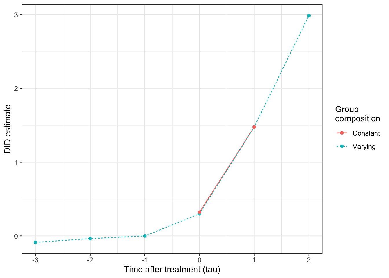

$DID estimates at various time periods after the treament aggregated across all treatment groups and maintaining treatment group composition constant (reference period $\tau'=1$)$

Figure 4.29: DID estimates at various time periods after the treament aggregated across all treatment groups and maintaining treatment group composition constant (reference period $\tau'=1$)

As expected, Figure 4.29 confirms that group composition does not play an important role in treatment effect heterogeneity: there actually is a true heterogeneity along the time dimension: the treatment effect seems to increase linearly over time (as we suspected it would, since we parameterized our model just like it).

Another plot that might prove very helpful is the one combining the aggregated estimates obtained in Figure 4.29 with the estimates obtained on each subgroup. This plot helps understand the source of heterogeneity in the profile of the aggregated treatment effects by attributing it to true treatment effect heterogeneity or to changes in group composition. Let’s go:

# building the dataset
DID.tau.agg.tot.inter <- DID.tau.agg.tot %>%
                    filter(Composition=="Varying") %>%
                    select(tau,ATT.tau.agg) %>%
                    rename(
                      ATT.tau=ATT.tau.agg
                    ) %>%
                    mutate(
                      d = "Aggregate",
                      prop.group=0
                    )

DID.tau <- rbind(DID.tau,DID.tau.agg.tot.inter) %>%
            mutate(
              d=factor(d,levels=c("2","3","4","Aggregate"))
            )

# plotting the result
ggplot(DID.tau,aes(x=tau,y=ATT.tau,colour=d,linetype=d))+
    geom_line() +
    geom_point() +
    ylab("DID estimate") +
    xlab("Time after treatment (tau)") +
    scale_x_continuous(breaks=c(-3,-2,-1,0,1,2)) +
    expand_limits(y=0) +
    scale_colour_discrete(name="Group\ncomposition")+
    scale_linetype_discrete(name="Group\ncomposition")+
    theme_bw()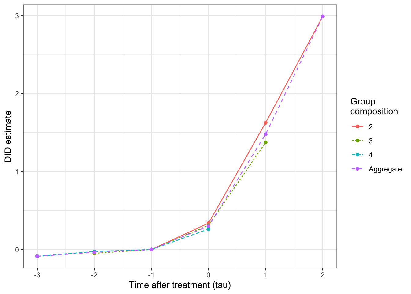

$DID estimates at various time periods after the treament aggregated across all treatment groups (reference period $\tau'=1$)$

Figure 4.30: DID estimates at various time periods after the treament aggregated across all treatment groups (reference period $\tau'=1$)

Finally, let us aggregate all treatment effects from all periods into one unique estimate. It is not an easy feat, especially in our current example which exhibits lots of treatment effect heterogeneity over $\tau$. Should we simply aggregate all treatment effect estimates using equal weights for each period $\tau$ or, rather, should we try to reflect the actual composition of treated groups and time periods in the sample? The choice of the mode of aggregation might make a huge difference to the eventual result, since giving more weights to higher $\tau$ will result in a much higher overall treatment effect. Let’s see what happens with both approaches.

# aggregating by weighing equally each time period tau
ATT.equal <- DID.tau.agg.tot %>%
                filter(Composition=="Varying",tau>=0) %>%
                summarize(
                  ATT.equal = mean(ATT.tau.agg)
                ) %>%
                pull(ATT.equal)

# aggregating by weighing as a proportion of time spent by each group in the treatment state 
ATT.varying <- DID.tau %>%
            ungroup() %>%
            filter(d!="Aggregate",tau>=0) %>%
            mutate(
              w.ATT = prop.group*ATT.tau
            ) %>%
            summarize(
              sum.w.ATT = sum(w.ATT),
              sum.w = sum(prop.group)
            ) %>% 
            mutate(
              ATT.varying = sum.w.ATT/sum.w
            ) %>%
            pull(ATT.varying)

The average effect of the treatment, giving equal weight to each time period $\tau\in\{0,1,2\}$, is equal to $\hat\Delta^{Y}_{TT}(e)=$ 1.59, where $e$ stands for “equal” weights. The average effect of the treatment, giving weights proportional to group composition and time spent in the treatment is equal to $\hat\Delta^{Y}_{TT}(v)=$ 1.06, where $v$ stands for “varying” weights.

4.3.3.2.2 Direct weighting using one reference period and one reference group (Sun and Abraham)

OK, so now, we know how to compute the various DID estimators by hand and how to aggregate them. Is there a way to obtain directly an aggregated estimate with an R package? Yes, actually, plenty of such estimator exist. They are listed on Asjad Naqvi’s DID webpage. Let’s start with the ones implementing the Sun and Abraham (2021) estimator. Sun and Abraham (2021)’s estimator start with estimating a Two Way Fixed Effect model with a rich dynamic specification:

\[\begin{align*} Y_{i,t} & = \mu_i + \delta_t + \sum_{d=2}^T\sum_{\tau\neq-1}\beta_{d,\tau}^{SA}\uns{D_{i}=d \land t=d+\tau} + \epsilon^{SA}_{i,t}, \end{align*}\]

on the sample excluding the always treated individuals ($D_i=1$). In order to be consistent with previous estimators, we are going to start using the fixest package to obtain our estimator. In order to be able to estimate Sun and Abraham (2021)’s estimator with fixest, we simply are going to add a sunab(d,t) term to the feols command, with the first term giving the treatment group and the second term the time fixed effect. We then can aggregate the estimated terms using regexp in order to detect the string patterns.

Example 4.43 Let’s go:

# regression
reg.fixest.SA.Agg <- feols(y ~ sunab(Ds,time)| id + time, data=filter(data,Ds>1))

# aggregate estimate (this is a command specific to fixest that aggregates various coefficients where an i. specification was used)
# The selection of coefficients to aggregate uses a string detection pattern language
# varying composition
aggregate.SA.varying <- aggregate(reg.fixest.SA.Agg, c("tau" = "time::([[:digit:]]+)"))

# another approach using the i function: not run, but works
# creating a time to treatment variable:
# data <- data %>%
#           mutate(
#             tau=time-Ds
#           ) %>%
#           mutate( 
#             tau = replace(tau,tau<=-90,-99)
#           )

# regression
# reg.fixest.SA.nonAgg <- feols(y ~ i(tau,i.Ds,ref=c(-1,-99))| id + time, data=filter(data,Ds>1))
# aggregate estimate (this is a command specific to fixest that aggregates various coefficients where an i. specification was used)
# The selection of coefficients to aggregate uses a string detection pattern language
# varying composition
# aggregate.SA.nonAgg.varying <- aggregate(reg.fixest.SA.nonAgg, c("tau" = "tau::([[:digit:]]+)"))

Let’s plot the results:

# preparation
colnames(aggregate.SA.varying) <- c("ATT","Se","t","pval")
aggregate.SA.varying <- aggregate.SA.varying %>%
                  as.data.frame(.)  %>%
                  mutate(tau = 0:2) 

# plot
ggplot(aggregate.SA.varying,aes(x=tau,y=ATT))+
    geom_line() +
    geom_pointrange(aes(ymin=ATT-1.96*Se,ymax=ATT+1.96*Se)) +
    ylab("DID estimate") +
    xlab("Time after treatment (tau)") +
    scale_x_continuous(breaks=c(0,1,2)) +
    expand_limits(y=0) +
    scale_colour_discrete(name="Group\ncomposition")+
    scale_linetype_discrete(name="Group\ncomposition")+
    theme_bw()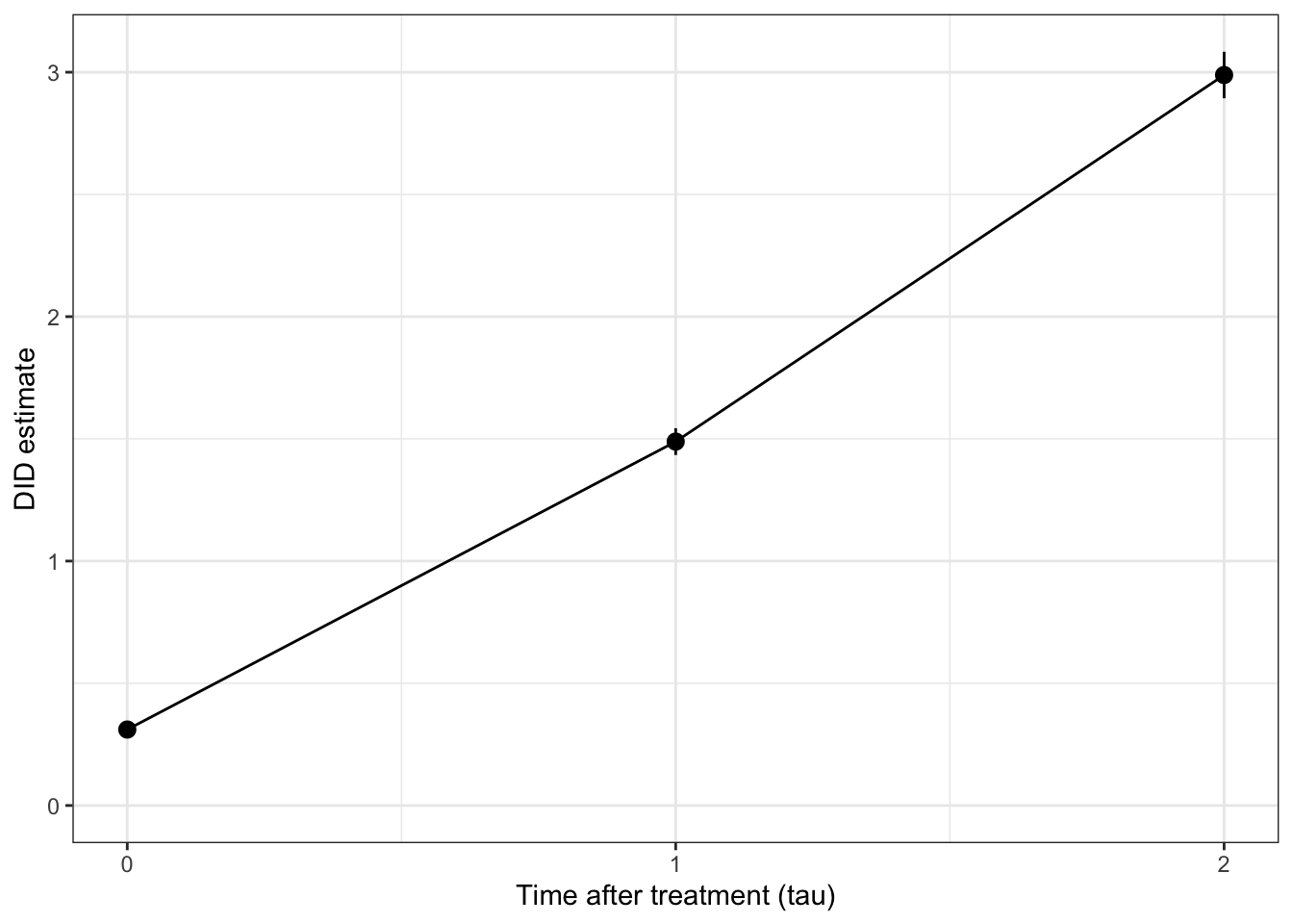

$DID estimates at various time periods after the treament using Sun and Abraham's estimator implemented by fixest (reference period $\tau'=1$)$

Figure 4.31: DID estimates at various time periods after the treament using Sun and Abraham’s estimator implemented by fixest (reference period $\tau'=1$)

Again, as we have seen before, the change in group composition makes it look like there is a trend break in the treatment effect. What we would need is to aggregate treatment effects with a constant group composition. One way to do that would be to use the full disaggregated results of the Sun and Abraham decomposition and to reaggregate them in another way. In order to access the disaggregated results of the Sun and Abraham regression, we need to use the option agg=FALSE in the coef and se commands. Let’s see how this works.

# Disaggregate estimates
disaggregate.SA <- as.data.frame(cbind(coef(reg.fixest.SA.Agg,agg=FALSE),se(reg.fixest.SA.Agg,agg=FALSE)))
colnames(disaggregate.SA) <- c('Coef','Se')
# adding treatment groups and time to treatment
disaggregate.SA <- disaggregate.SA %>%
                    mutate(test =  names(coef(reg.fixest.SA.Agg,agg=FALSE))) %>%
                    mutate(
                      Group = factor(str_sub(test,-1),levels=c('1','2','3','4','Aggregate')),
                      TimeToTreatment = factor(if_else(str_detect(test,"\\-"),str_extract(test,"\\-[[:digit:]]"),str_extract(test,"[[:digit:]]")),levels=c('-3','-2','-1','0','1','2'))
                    ) %>%
                  select(-test)

# adding reference period
Group <- c('2','3','4')
TimeToTreatment <- rep('-1',3)
ref.dis <- as.data.frame(cbind(Group,TimeToTreatment)) %>%
        mutate(
          Coef = 0,
          Se = 0,
          Group = factor(Group,levels=c('1','2','3','4','Aggregate')),
          TimeToTreatment = factor(TimeToTreatment,levels=c('-3','-2','-1','0','1','2'))
          )
disaggregate.SA <- rbind(disaggregate.SA,ref.dis) 

# adding aggregate results
# aggregate estimates
aggregate.SA <- as.data.frame(cbind(coef(reg.fixest.SA.Agg),se(reg.fixest.SA.Agg)))
colnames(aggregate.SA) <- c('Coef','Se')
# adding treatment groups and time to treatment
aggregate.SA <- aggregate.SA %>%
                    mutate(test =  names(coef(reg.fixest.SA.Agg))) %>%
                    mutate(
                      Group = factor(rep("Aggregate",5),levels=c('1','2','3','4','Aggregate')),
                      TimeToTreatment = factor(if_else(str_detect(test,"\\-"),str_extract(test,"\\-[[:digit:]]"),str_extract(test,"[[:digit:]]")),levels=c('-3','-2','-1','0','1','2'))
                    ) %>%
                  select(-test)

# adding reference period
Group <- c("Aggregate")
TimeToTreatment <- rep('-1',1)
ref <- as.data.frame(cbind(Group,TimeToTreatment)) %>%
        mutate(
          Coef = 0,
          Se = 0,
          Group = factor(Group,levels=c('1','2','3','4','Aggregate')),
          TimeToTreatment = factor(TimeToTreatment,levels=c('-3','-2','-1','0','1','2'))
          )
disaggregate.SA <- rbind(disaggregate.SA,aggregate.SA,ref) %>%
                    mutate(TimeToTreatment = as.numeric(as.character(TimeToTreatment)))

Let’s plot the result:

ggplot(disaggregate.SA,aes(x=TimeToTreatment,y=Coef,colour=Group,linetype=Group))+
    geom_line() +
    geom_pointrange(aes(ymin=Coef-1.96*Se,ymax=Coef+1.96*Se)) +
    ylab("DID estimate") +
    xlab("Time relative to treatment") +
    scale_x_continuous(breaks=c(-3,-2,-1,0,1,2)) +
    expand_limits(y=0) +
    scale_colour_discrete(name="Treatment\ngroup")+
    scale_linetype_discrete(name="Treatment\ngroup")+
    theme_bw()

$Disaggregated DID estimates around the treatment date estimated using the Sun and Abraham procedure in fixest (reference period $\tau'=1$)$

Figure 4.32: Disaggregated DID estimates around the treatment date estimated using the Sun and Abraham procedure in fixest (reference period $\tau'=1$)

Figure 4.32 shows very well how the Sun and Abraham estimator works: it aggregates each group specific treatment effect (relative to the reference period $\tau'=-1$ and to the reference group ($D_i=\infty$)) with period-specific weights which depend on the proportion of each treated group among the treated at this period. As a result, some dynamic changes in treatment effects might be driven by changes in group composition and not by genuine changes in the effect of the treatment. This is the case in Figure 4.32 between periods 1 and 2 where the acceleration in the growth of the aggregated treatment effect is due to the disappearance of group 3, which has a lower speed of increase of its average treatment effect, at period 2. As it is always tricky to interpret the aggregated result, I suggest to always plot the disaggregated results on the same graph, as in Figure 4.32.

Let us finally compute the aggregated effect:

ATT.agg.SA <- aggregate(reg.fixest.SA.Agg, c("ATT" = "time::[^-]"))

The aggregated effect estimated using the Sun and Abraham approach as implemented in fixest is equal to 1.07 $\pm$ 0.04.

Remark. Sun and Abraham’s estimator can also be formulated in repeated cross sections by estimating the following model by OLS:

\[\begin{align*} Y_{i,t} & = \alpha + \sum_{d=2}^T\mu_d\uns{D_{i}=d} + \sum_{\tau=2}^{T}\delta_{\tau}\uns{t=\tau} + \sum_{d=2}^T\sum_{\tau\neq-1}\beta_{d,\tau}^{SA}\uns{D_{i}=d \land t=d+\tau} + \epsilon^{SA}_{i,t}. \end{align*}\]

Remark. We can also show that Sun and Abraham’s estimator is equal to our individual DID estimators in the population:

Theorem 4.19 (Sun and Abraham estimator is equivalent to individual DID in the population) In the population, Sun and Abraham’s estimator (formulated in a panel and in a repeated cross section) is equal to the individual DID estimators using the never treated as the comparison group and the period just before receiving the treatment as the reference period: $\forall d\in\left\{2,\dots,T\right\}$, $\forall\tau\in\left\{-(T-1),\dots,T-2\right\}\setminus\left\{-1\right\}$,

\[\begin{align*} \beta_{d,\tau}^{SA} & = \Delta^{Y}_{DID}(d,\infty,\tau,d-1). \end{align*}\]

Proof. See Section A.3.3.

Remark. We can also show that Sun and Abraham’s estimator is equal to our individual DID estimators in the sample:

Theorem 4.20 (Sun and Abraham estimator is equivalent to individual DID in the sample) In the sample, Sun and Abraham’s estimator (estimated by OLS in repeated cross sections or in panel data or by OLS using the Least Squares Dummy Variables model, the Within transformation or the First Difference transformation relative to $d-1$ in panel data) is equal to the individual DID estimators using the never treated as the comparison group and the period just before receiving the treatment as the reference period: $\forall d\in\left\{2,\dots,T\right\}$, $\forall\tau\in\left\{-(T-1),\dots,T-2\right\}\setminus\left\{-1\right\}$,

\[\begin{align*} \hat{\beta}_{d,\tau}^{SA} & = \frac{\sum_{i=1}^{N_{d+\tau}}Y_{i,d+\tau}\uns{D_i=d}}{\sum_{i=1}^{N_{d+\tau}}\uns{D_i=d}} -\frac{\sum_{i=1}^{N_{d-1}}Y_{i,d-1}\uns{D_i=d}}{\sum_{i=1}^{N_{d-1}}\uns{D_i=d}} \\ & \phantom{=} - \left(\frac{\sum_{i=1}^{N_{d+\tau}}Y_{i,d+\tau}\uns{D_i=\infty}}{\sum_{i=1}^{N_{d+\tau}}\uns{D_i=\infty}} -\frac{\sum_{i=1}^{N_{d-1}}Y_{i,d-1}\uns{D_i=\infty}}{\sum_{i=1}^{N_{d-1}}\uns{D_i=\infty}}\right) \end{align*}\]

Proof. See Section A.3.4.

Remark. The First Difference transformation of the Sun and Abraham model that is equivalent to the individual DID estimator is not a standard first difference where observations observed at date $t-1$ are subtracted from observations at $t$. The correct First Difference transformation is relative to $d-1$: the OLS regression is performed on the following model, restricted to the sample where $D_i=d$ or $D_i=\infty$ and $T_i=t$ or $T_i=d-1$:

\[\begin{align*} D_j^{d,\tau}(Y_{j,d+\tau} - Y_{j,d-1}) & = \alpha_{d,\tau}^{FD}D_j^{d,\tau} + \beta_{d,\tau}^{FD}\uns{D_j=d}D_j^{d,\tau} + \epsilon^{FD}_{j,t}D_j^{d,\tau}, \end{align*}\]

where $D_j^{d,\tau}$ takes value one when observation $j$ is used to estimate $\hat\beta^{SA}_{d,\tau}$.

Example 4.44 In order to see how Theorem 4.20 works in practice, let us collect all the estimated effects obtained thanks to our separate individual DID estimators and compare them with the coefficients of Sun and Abraham’s model.

We are going to compare the coefficients in the Sun and Abraham model to the DID estimates that compare each treated group to the never treated group, since the Sun and Abraham estimator do not use the observations belonging to groups that eventually get treated as controls when they are not yet treated.

# reorganize the DID estimator
DID.1.mod <- DID.1 %>%
          filter(dprime=="99") %>% # keep only never treated as counterfactuals
          rename(
            TimeToTreatment=tau,
             Group=d
          ) %>%
          mutate(
            Group=factor(Group,levels=c("1","2","3","4","Aggregate")),
            TimeToTreatment=as.numeric(TimeToTreatment)
          ) %>%
          select(DIDest,DIDse,Group,TimeToTreatment)

# add reference period to DID estimator
DID.1.mod <- rbind(DID.1.mod,ref.dis %>% rename(DIDest=Coef,DIDse=Se)) %>%
          mutate(
            TimeToTreatment=as.numeric(TimeToTreatment)
          )

# joining DID and SA estimates
CompDIDSA <- DID.1.mod %>%
              left_join(disaggregate.SA,by=c('Group','TimeToTreatment')) %>%
                 mutate(
                     TimeToTreatment = factor(TimeToTreatment,levels=c('-3','-2','-1','0','1','2'))
                 )

Let’s now plot the results:

ggplot(CompDIDSA,aes(x=DIDest,y=Coef,shape=Group,color=TimeToTreatment))+
    geom_point() +
    geom_abline(slope=1,intercept=0,linetype="dotted",color="red")+
    ylab("Sun and Abraham estimate") +
    xlab("DID estimate") +
    theme_bw()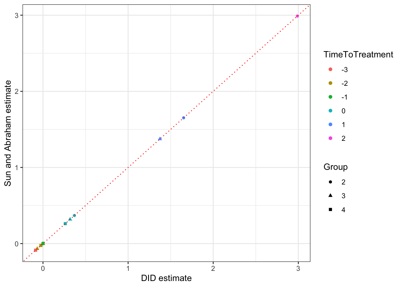

$Comparison of treatment effects estimated using DID and Sun and Abraham estimator (reference period $\tau'=1$)$

Figure 4.33: Comparison of treatment effects estimated using DID and Sun and Abraham estimator (reference period $\tau'=1$)

As Figure 4.33 shows, the coefficients estimated through DID are identical to the coefficients estimated using Sun and Abraham approach (they all lone up on the 45 degree line). This is an illustration of the main result of Theorem 4.20.

Note that the estimated aggregated effect using DID with weights proportional to group composition and time spent in the treatment is equal to $\hat\Delta^{Y}_{TT}(v)=$ 1.06. The corresponding estimate using Sun and Abraham estimator is equal to 1.07 $\pm$ 0.04. The two estimator are slightly different. This is because Sun and Abraham aggregate effects estimated using exclusively the never treated group as the control group while the DID estimator aggregates the same and effects estimated using the other treated groups before they receive the treatment. It should be the case that if we aggregate the DID estimates using only the never treated as the control group, we should obtain the same result as with Sun and Abraham estimator. Let’s check.

# joining the weights to the results
DID.1.agg.SA <- DID.1 %>%
                  filter(dprime=="99",tau>=0) %>%
                  select(-prop.group) %>%
                  mutate(
                    d= factor(d,levels=c("99","4","3","2","1"))
                  ) %>%
                  left_join(prop.groups.DID,by=c("d"="dprime")) %>% 
                  mutate(
                    w.ATT = prop.group*DIDest
                  ) %>%
                  summarize(
                    sum.w.ATT = sum(w.ATT),
                    sum.w = sum(prop.group)
                  ) %>% 
                  mutate(
                    ATT.varying.DID = sum.w.ATT/sum.w
                  ) %>%
                  pull(ATT.varying.DID)

The estimated aggregated effect using DID with weights proportional to group composition and time spent in the treatment, restricting the estimates to the ones obtained using the never treated as the control group is equal to $\hat\Delta^{Y}_{TT}(v)=$ 1.07, which is indeed equal to the aggregate estimate computed by the Sun and Abraham estimator in fixest.

Remark. What to do in pratice? Use only the never treated as controls?
It seems that using more groups as controls (if they are valid) should increase efficiency.

4.3.3.2.3 Direct weighting using one reference period and one reference group (Callaway and Sant’Anna)

Callaway and Sant’Anna (2021) propose an alternative estimator to the one proposed by Sun and Abraham. They suggest using a doubly robust matching estimator to condition on observed covariates. We are only going to encouter these estimators in Section ??. In the absence of covariates, Callaway and Sant’Anna’s estimator is equivalent to the Sun and Abraham estimator. Callaway and Sant’Anna have proposed the did package to implement their estimator. The main command is att_gt, which computes all the estimates for each treatment group $D_i=g$ and each time period $t$.

Example 4.45 Let’s see if we can make it work.

# preparing the data
# The Group variable has to take value 0 for the never treated (instead of infty or 99)
data <- data %>%
          mutate(
            Group = if_else(Ds<99,Ds,0)
          )

# regression
reg.CSA <- att_gt(yname="y",tname="time",idname="id",gname="Group",data=filter(data,Ds!=1),base_period="universal")

# dynamic treatment effects (event-study graph)
reg.CSA.Agg <- aggte(reg.CSA,type="dynamic")

Let’s plot the result:

# preparing the results for the plot  
DID.CSA <- as.data.frame(reg.CSA$group)
colnames(DID.CSA) <- c("Group")
DID.CSA <- DID.CSA %>%
            mutate(
              time = reg.CSA$t,
              Coef = reg.CSA$att,
              Se = reg.CSA$se
            ) %>%
            mutate(
              TimeToTreatment = time-Group,
              Group = factor(Group,levels=c('1','2','3','4','Aggregate')),
            )

# add aggregate effect
DID.CSA.Agg <- as.data.frame(cbind(reg.CSA.Agg$egt,reg.CSA.Agg$att.egt,reg.CSA.Agg$se.egt))
colnames(DID.CSA.Agg) <- c('TimeToTreatment','Coef','Se')
DID.CSA.Agg <- DID.CSA.Agg %>%
                mutate(
                  Group = factor(rep("Aggregate",nrow(DID.CSA.Agg)),levels=c('1','2','3','4','Aggregate'))
                )

# merge all results
DID.CSA <- rbind(select(DID.CSA,-time),DID.CSA.Agg)

ggplot(DID.CSA,aes(x=TimeToTreatment,y=Coef,colour=Group,linetype=Group))+
    geom_line() +
    geom_pointrange(aes(ymin=Coef-1.96*Se,ymax=Coef+1.96*Se)) +
    ylab("DID estimate") +
    xlab("Time relative to treatment") +
    scale_x_continuous(breaks=c(-3,-2,-1,0,1,2)) +
    expand_limits(y=0) +
    scale_colour_discrete(name="Treatment\ngroup")+
    scale_linetype_discrete(name="Treatment\ngroup")+
    theme_bw()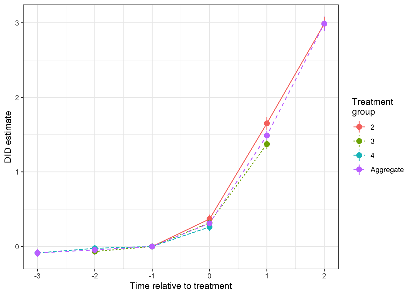

$Disaggregated DID estimates around the treatment date estimated using the Callaway and Sant'Anna procedure in did (reference period $\tau'=1$)$

Figure 4.34: Disaggregated DID estimates around the treatment date estimated using the Callaway and Sant’Anna procedure in did (reference period $\tau'=1$)

Figure 4.34 shows a result that is very similar to the one obtained in Figure 4.32 using Sun and Abraham’s approch as implemented in fixest. The two approaches are indeed equivalent with the options that we have chosen.

Let us finally compute the aggregated treatment effect:

ATT.agg.CSA <- aggte(reg.CSA,type="simple")

The aggregated effect estimated using the Callaway and Sant’Anna approach as implemented in did is equal to 1.07 $\pm$ 0.06.

4.3.3.2.4 De Chaisemartin and d’Haultfoeuille

de Chaisemartin et d’Haultfoeuille propose two ways to deal with DID with differences in treatment timing. In de Chaisemartin and d’Haultfoeuille (2020), they propose to estimate the effect of the treatment using only the periods where a change in treatment status occurs, by comparing the treated to the not yet treated at the same time periods. In de Chaisemartin et d’Haultfoeuille (2021), they propose to estimate the dynamic effect of the treatment using a discounted sum of treatment effects over time. In its simplest form, with staggered designs, a discrete treatment and no covariates, de Chaisemartin et d’Haultfoeuille (2021)’s estimator is equivalent to that of Sun and Abraham or Callaway and Sant’Anna. Both estimators have been implemented in the DIDmutiplegt package with the did_multiplegt function.

Example 4.46 Let’s see how it works.

# regression
reg.dCdH <- did_multiplegt(Y="y",T="time",G="id",D="D",df=filter(data,Ds!=1),placebo=3,dynamic=3,average_effect="prop_number_switchers")

Let us now pot the results:

# preparing the results for the plot  
DID.dCdH <- as.data.frame(c(reg.dCdH$placebo_2,reg.dCdH$placebo_1,0,reg.dCdH$effect,reg.dCdH$dynamic_1,reg.dCdH$dynamic_2))
colnames(DID.dCdH) <- c("Coef")
DID.dCdH <- DID.dCdH %>%
            mutate(
              TimeToTreatment = c(-3,-2,-1,0,1,2),
              Se = c(reg.dCdH$se_placebo_2,reg.dCdH$se_placebo_1,0,reg.dCdH$se_effect,reg.dCdH$se_dynamic_1,reg.dCdH$se_dynamic_2)
            ) 

ggplot(DID.dCdH,aes(x=TimeToTreatment,y=Coef))+
    geom_line() +
    geom_pointrange(aes(ymin=Coef-1.96*Se,ymax=Coef+1.96*Se)) +
    ylab("DID estimate") +
    xlab("Time relative to treatment") +
    scale_x_continuous(breaks=c(-3,-2,-1,0,1,2)) +
    expand_limits(y=0) +
    theme_bw()

$DID estimates around the treatment date estimated using the de Chaisemartin and d'Haultfoeuille procedure (reference period $\tau'=1$)$

Figure 4.35: DID estimates around the treatment date estimated using the de Chaisemartin and d’Haultfoeuille procedure (reference period $\tau'=1$)

Figure 4.35 shows that the profile estimated using de Chaisemartin and d’Haultfoeuille’s aprproach is similar but distinct from the one estimated by the other authors. Why is still to be determined.

Finally, the aggregate efect of the treatment as estimated by the de Chaisemartin and d’Haultfoeuille (2020) approach is equal to 0.3. I have been unable to obtain standard errors for this estimator for now.

4.3.3.2.5 Imputation methods: Borusyak, Jaravel and Speiss

Borusyak, Jaravel and Speiss (2021) adopt a very different framework from the previous ones. They do not build from the individual DID estimators $\Delta^{Y}_{DID}(d,d',\tau,\tau')$, but instead propose to estimate the individual level treatment effects $\hat\Delta^Y_{i,t}$ and then to aggregate them as one wishes to. In order to build an estimate of the individual level treatment effects $\hat\Delta^Y_{i,t}$, Borusyak, Jaravel and Speiss (2021) propose to use an imputation estimator, $\hat Y^0_{i,t}$, which predicts the value of $Y^0_{i,t}$ for each treated unit. Borusyak, Jaravel and Speiss (2021)’s imputation estimator works as follows:

Within the never treated and not-yet-treated observations only, estimate $\hat\mu_i^{OLS}$ and $\hat\delta_t^{OLS}$ using the following OLS regression:

\[\begin{align*} Y^0_{i,t} & = \mu_i + \delta_t + U^0_{i,t} \end{align*}\]

For each treated observation, set $\hat Y^0_{i,t} = \hat\mu_i^{OLS}+\hat\delta_t^{OLS}$ and $\hat\Delta^Y_{i,t}=Y^1_{i,t}-\hat Y^0_{i,t}$.

Finally, Borusyak, Jaravel and Speiss (2021) propose to aggregate the estimates for each treatment effect using weights $w^{BJS_k}_{i,t}$ in order to form $\hat\Delta^{Y}_{TT}(BJS_k)=\sum w^{BJS_k}_{i,t}\hat\Delta^Y_{i,t}$.

In the absence of covariates, or group-specific time trends, the main assumption of Borusyak, Jaravel and Speiss (2021)’s framework is that the potential outcomes in the absence of the treatment can be decomposed in two separate influences:

Hypothesis 4.26 (Additive Separability of Potential Outcomes in the Absence of the Treatment) We assume that the potential outcomes in the absence of the treatment are additively separable between time and individual fixed effects:

\[\begin{align*} Y^0_{i,t} & = \mu_i + \delta_t + U^0_{i,t}, \end{align*}\]

with $\esp{U^0_{i,t}|D_i}=0$, $\forall t\in\{1,\dots,T\}$.

Assumption 4.26 assumes that all the time and individual-level influences on potential outcomes that are potentially correlated with treatment intake are additively separable.

Remark. Borusyak, Jaravel and Speiss (2021) claim that Assumption 4.26 is equivalent to Assumption 4.25 of parallel trends. I think we still need a formal proof of that claim.

Borusyak, Jaravel and Speiss (2021) add another assumption, namely that error terms are homoskedastic:

Hypothesis 4.27 (Homoskedasticity) We assume that the error terms are homoskedastic and mutually uncorrelated:

\[\begin{align*} \esp{U_0U_0'} & = \sigma^2\mathbf{I}, \end{align*}\]

with $U_0$ the vector of error terms and $\mathbf{I}$ the identity matrix of the coresponding dimension.

Under these assumptions, and the no-anticipation condition, Borusyak, Jaravel and Speiss (2021) prove a very powerful result:

Theorem 4.21 (Imputation identifies Weighted TT) Under Assumptions 4.23, 4.24 and 4.26, the imputation estimator is the unique efficient linear unbiased estimator of the corresponding weighted average of Treatment on the Treated:

\[\begin{align*} \sum w^{BJS_k}_{i,t}\hat\Delta^Y_{i,t} & = \Delta^{Y}_{TT}(BJS_k). \end{align*}\] with \[\begin{align*} \Delta^{Y}_{TT}(BJS_k) & = \sum w^k_{i,t}\Delta^Y_{i,t} \end{align*}\]

Proof. See Borusyak, Jaravel and Speiss (2021) Theorems 1 and 2.

Theorem 4.21 is a pretty cool result. It shows that, under the assumptions made so far, the imputation estimator is the most efficient way to combine observations in order to obtain DID estimates of the effect of the treatment.

Remark. The “trick” that makes the Borusyak, Jaravel and Speiss (2021)’s imputation estimator more efficient than Sun and Abraham or Callaway and Sant’Anna’s estimators is that it combines all pre-treatment observations when generating the treatment effect estimate. An open question is whether a weigthed average of the individual DID estimates, including all the ones formed using all pre-treatment observations as reference periods, is as efficient as Borusyak, Jaravel and Speiss (2021)’s imputation estimator.

Remark. Borusyak, Jaravel and Speiss (2021) claim that Assumption 4.27 can be relaxed to any known form of heteroskedasticity or autocorrelation and that Theorem 4.21 would still hold.

How does Borusyak, Jaravel and Speiss (2021)’s imputation estimator work in practice? Thanks to the amazing Kyle Butts, we have a package that computes Borusyak, Jaravel and Speiss (2021)’s imputation estimator, didimputation. The command is did_imputation.

Example 4.47 Let’s see how it works.

# regression
reg.BJS <- did_imputation(yname="y",tname="time",idname="id",gname="Group",data=filter(data,Ds!=1),horizon=TRUE,pretrends=TRUE)

Let us now plot the results:

# preparing the results for the plot  
DID.BJS <- reg.BJS %>%
            rename(
              TimeToTreatment=term,
              Coef=estimate,
              Se=std.error
            ) %>%
            mutate(
              TimeToTreatment=as.numeric(TimeToTreatment)
            )
# adding reference period
DID.BJS[nrow(DID.BJS)+1,] <- list(-1,0,0,0,0)

#plot
ggplot(DID.BJS,aes(x=TimeToTreatment,y=Coef))+
    geom_line() +
    geom_pointrange(aes(ymin=Coef-1.96*Se,ymax=Coef+1.96*Se)) +
    ylab("DID estimate") +
    xlab("Time relative to treatment") +
    scale_x_continuous(breaks=c(-3,-2,-1,0,1,2)) +
    expand_limits(y=0) +
    theme_bw()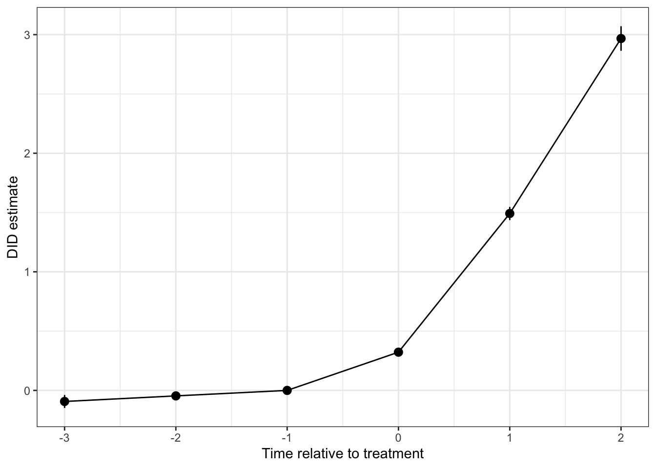

$DID estimates around the treatment date estimated using Borusyak, Jaravel and Speiss's procedure (reference period $\tau'=1$)$

Figure 4.36: DID estimates around the treatment date estimated using Borusyak, Jaravel and Speiss’s procedure (reference period $\tau'=1$)

As Figure 4.36 shows, the dynamic profile of the treatment effect estimated using Borusyak, Jaravel and Speiss’s procedure is very similar to the one obtained using Sun and Abraham and Callaway and Sant’Anna.

Let us finally estimate the average treatment effect on the treated using Borusyak, Jaravel and Speiss’s procedure:

# regression
reg.BJS.Agg <- did_imputation(yname="y",tname="time",idname="id",gname="Group",data=filter(data,Ds!=1))

The treatment effect estimated using Borusyak, Jaravel and Speiss’s estimator is equal to 1.08 $\pm$ 0.04.

4.3.3.2.6 Imputation methods: Gardner

Gardner (2021) proposes a two stage estimator very similar to the one by Borusyak, Jaravel and Speiss (2021). Gardner writes outcomes for individual $i$ at time $t$ as follows, with group and time fixed effects:

\[\begin{align*} Y_{i,t} & = \sum_{d=1}^{\infty}\lambda_d\uns{D_i=d} + \sum_{l=1}^T\delta_l\uns{l=t} + \sum_{d=1}^{\infty}\sum_{l=1}^T\beta^G_{d,l}\uns{D_i=d}\uns{l=t} + \epsilon^{G}_{i,t}, \end{align*}\]

where the groups are defined by the date at which they start receiving the treatment. In practice, Gardner’s estimator works as follows:

Estimate the following model using OLS on the sample of observations for which $D_{i,t}=0$ (which excludes all the currently treated):

\[\begin{align*} Y_{i,t} & = \sum_{d=2}^{\infty}\lambda_d\uns{D_i=d} + \sum_{l=1}^T\delta_l\uns{l=t} + \epsilon^{G}_{i,t} \end{align*}\]

Regress the adjusted outcomes $Y_{i,t}-\sum_{d=2}^{\infty}\hat\lambda_d\uns{D_i=d}-\sum_{l=1}^T\hat\delta_l\uns{l=t}$ on $D_{i,t}$ and retain the coefficient $\hat\beta^G$. Note as well that one can also estimate the average effect of the treatment around each treatment date by regressing the adjusted outcomes on a set of dummies taking value one when observation $i$ at period $t$ is $\tau$ periods from the treatment (here, we omit the dummy for the never treated group and for one reference period, in general $\tau=-1$).

Gardner shows that the coefficient on $D_{i,t}$ in the second stage of this procedure ($\hat\beta^G$) identifies the average effect of the treatment on the treated under the usual parallel trends assumptions: $\beta^G=\esp{\Delta^Y_{i,t}|D_{i,t}=1}$, where $\Delta^Y_{i,t}=Y^1_{i,t}-Y^0_{i,t}$. What is pretty great is that Gardner, together with Kyle Butts, have provided an R package in order to perform the estimation: did2s.

Example 4.48 Let’s see how it works in our example.

# regression
reg.Gardner <- did2s(data=filter(data,Ds!=1),yname = "y", first_stage = ~ 0 | id + time,second_stage = ~i(D, ref=FALSE), treatment = "D",cluster_var = "id")

The overall estimated treatment effect is 1.08 $\pm$ 0.06. This seems valid enough. Now, did2s also provides a way to estimate the effect at each time period relative the treatment date (a.k.a. the event study estimates).

# generating a TimeToTreatment variable
data <- data %>%
          mutate(
            TimeToTreatment = if_else(abs(time-Ds)<90,time-Ds,-99)
          )

# regression
reg.Gardner.event.study <- did2s(data=filter(data,Ds!=1),yname = "y", first_stage = ~ 0 | id + time,second_stage = ~i(TimeToTreatment, ref=c(-1, -99)), treatment = "D",cluster_var = "id")

Let us now plot the results:

# putting results into a dataframe
resultsGardnerEventStudy <- as.data.frame(cbind(coef(reg.Gardner.event.study),se(reg.Gardner.event.study)))
colnames(resultsGardnerEventStudy) <- c('Coef','Se')
# adding the time to treatment variable
resultsGardnerEventStudy <- resultsGardnerEventStudy %>%
                              mutate(
                                TimeToTreatment = c(-3,-2,0,1,2)
                              )
# adding the reference period
resultsGardnerEventStudy <- rbind(resultsGardnerEventStudy,c(0,0,-1))

#plot
ggplot(resultsGardnerEventStudy,aes(x=TimeToTreatment,y=Coef))+
    geom_line() +
    geom_pointrange(aes(ymin=Coef-1.96*Se,ymax=Coef+1.96*Se)) +
    ylab("DID estimate") +
    xlab("Time relative to treatment") +
    scale_x_continuous(breaks=c(-3,-2,-1,0,1,2)) +
    expand_limits(y=0) +
    theme_bw()

$DID estimates around the treatment date estimated using Gardner's procedure (reference period $\tau'=1$)$

Figure 4.37: DID estimates around the treatment date estimated using Gardner’s procedure (reference period $\tau'=1$)

4.3.3.2.7 Imputation methods: Liu, Wang and Xu

Liu, Wang and Xu (2021) also propose a series of imputation estimators, with some very similar to the ones proposed by Borusyak, Jaravel and Speiss and by Gardner. Their Proposition 1 is very close to Theorem 4.21, albeit they do not prove that their estimator is the most efficient among linear estimators. They also propose an R package to estimate their estimators, fect. I will come back to this package later, in Section ??, since most of the estimators they propose try to relax the parallel trends assumption.

4.3.3.2.8 Stacked DID

The stacked DID approach has been proposed by Cengiz, Dube, Lindner and Zipperer (2019) and extended by Gardner (2021). For stacked DID, one creates a dataset for each group defined by its date of treatment, with all observations treated at that date and the ones that are not yet treated, one then stacks all these datasets together, and estimates a two-way fixed effects model with time $\times$ dataset specific fixed effects and individual fixed effects. Gardner’s Appendix A show that this procedure yields a weighted average of group and time specific treatment effects, with weights that do not generally correspond to the ones of the ATT estimate, but that are positive and sum to one. One issue I have with this approach is that it focuses only on cases where there are no never treated observations. If we keep never treated observations in the stacked DID approach, they are going to be used multiple times and one certainly needs to account for that when estimating precision.

The way I’m choosing to implement this approach is by adding specific group $\times$ time dummies for all the members of a given group defined by its date of first treatment and all the not-yet-treated observations at that same date. We are going to run a two-way fixed effects model on these fixed effects and on individual fixed effects as well as on treatment dummies.

Example 4.49 Let’s see how it goes.

# generating the groups x time dummies
data <- data %>%
          mutate(
            FE.1.1 = if_else(time ==1 & (Ds==1 | D==0),1,0),
            FE.1.2 = if_else(time ==2 & (Ds==1 | D==0),1,0),
            FE.1.3 = if_else(time ==3 & (Ds==1 | D==0),1,0),
            FE.1.4 = if_else(time ==4 & (Ds==1 | D==0),1,0),
            FE.2.1 = if_else(time ==1 & (Ds==2 | D==0),1,0),
            FE.2.2 = if_else(time ==2 & (Ds==2 | D==0),1,0),
            FE.2.3 = if_else(time ==3 & (Ds==2 | D==0),1,0),
            FE.2.4 = if_else(time ==4 & (Ds==2 | D==0),1,0),
            FE.3.1 = if_else(time ==1 & (Ds==3 | D==0),1,0),
            FE.3.2 = if_else(time ==2 & (Ds==3 | D==0),1,0),
            FE.3.3 = if_else(time ==3 & (Ds==3 | D==0),1,0),
            FE.3.4 = if_else(time ==4 & (Ds==3 | D==0),1,0),
            FE.4.1 = if_else(time ==1 & (Ds==4 | D==0),1,0),
            FE.4.2 = if_else(time ==2 & (Ds==4 | D==0),1,0),
            FE.4.3 = if_else(time ==3 & (Ds==4 | D==0),1,0),
            FE.4.4 = if_else(time ==4 & (Ds==4 | D==0),1,0)
          )

# regression for individual parameter
reg.stacked.aggregate <- feols(y ~ D 
                                  + FE.1.1 + FE.1.2 + FE.1.3 + FE.1.4
                                  + FE.2.1 + FE.2.2 + FE.2.3 + FE.2.4
                                  + FE.3.1 + FE.3.2 + FE.4.3 + FE.4.4
                               | id + time, data=filter(data,Ds!=1))

# event study regression
reg.stacked.event.study <- feols(y ~ i(TimeToTreatment,ref=c(-99,-1))
                                  + FE.1.1 + FE.1.2 + FE.1.3 + FE.1.4
                                  + FE.2.1 + FE.2.2 + FE.2.3 + FE.2.4
                                  + FE.3.1 + FE.3.2 + FE.4.3 + FE.4.4
                               | id + time, data=filter(data,Ds!=1))

The total estimate given by the stacked regression is of 1.86, which seems pretty large compared to the other estimators. Remember that the average effect of the treatment, giving equal weight to each time period $\tau\in\{0,1,2\}$, is equal to $\hat\Delta^{Y}_{TT}(e)=$ 1.59 while the average effect of the treatment, giving weights proportional to group composition and time spent in the treatment is equal to $\hat\Delta^{Y}_{TT}(v)=$ 1.06. Let us plot the corresponding results of the event study regression.

# putting results into a dataframe
resultsStackedDIDEventStudy <- as.data.frame(cbind(reg.stacked.event.study$coefficients[1:5],reg.stacked.event.study$se[1:5]))
colnames(resultsStackedDIDEventStudy) <- c('Coef','Se')
# adding the time to treatment variable
resultsStackedDIDEventStudy <- resultsStackedDIDEventStudy %>%
                              mutate(
                                TimeToTreatment = c(-3,-2,0,1,2)
                              )
# adding the reference period
resultsStackedDIDEventStudy <- rbind(resultsStackedDIDEventStudy,c(0,0,-1))

#plot
ggplot(resultsStackedDIDEventStudy,aes(x=TimeToTreatment,y=Coef))+
    geom_line() +
    geom_pointrange(aes(ymin=Coef-1.96*Se,ymax=Coef+1.96*Se)) +
    ylab("DID estimate") +
    xlab("Time relative to treatment") +
    scale_x_continuous(breaks=c(-3,-2,-1,0,1,2)) +
    expand_limits(y=0) +
    theme_bw()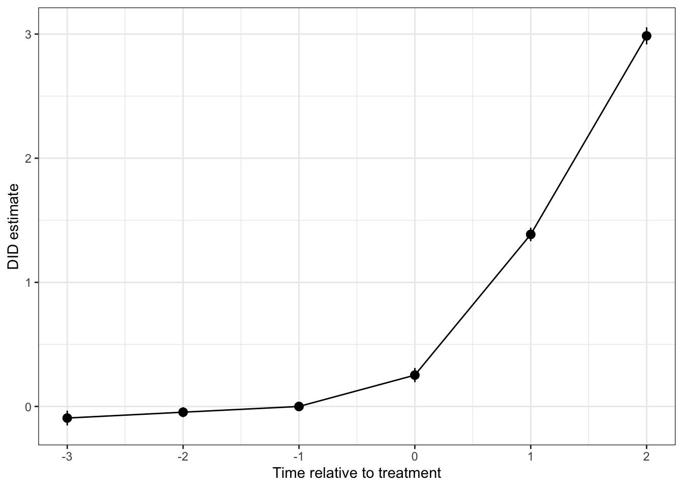

$DID estimates around the treatment date estimated using Stacked DID (reference period $\tau'=1$)$

Figure 4.38: DID estimates around the treatment date estimated using Stacked DID (reference period $\tau'=1$)

The results seem pretty nice and close to what we have obtained so far with the other methods we have used.

4.3.3.2.9 Two-Way Fixed Effects

Before we conclude, there is one last set of methods that we might have wanted to use: the methods based on the standard Two Way Fixed Effects model with time and unit-specific fixed effects that we have introduced in Sections 4.3.1.2.4, 4.3.1.2.5 and 4.3.1.2.6, and which can be estimated using various types of methods (Least Squares Dummy Variables, Within regression or other fast methods). Methods based on the Two Way Fixed Effects model were actually the most used ones to estimate treatment effects and event study regressions in staggered designs before a string of results showed that they had severe issues. In this section, we will cover the basic issues that methods based on the Two Way Fixed Effects model face in a staggered design and we will state conditions under which they can be correct.

Example 4.50 Before that, let us simply look at how the Two Way Fixed Effects model performs in our example.

# regression for individual parameter
reg.TWFE.aggregate <- feols(y ~ D | id + time, data=data)

# event study regression
reg.TWFE.event.study <- feols(y ~ i(TimeToTreatment,ref=c(-99,-1)) | id + time, data=data)

The Two Way Fixed Effects-based estimate of the aggregate treatment effect on the treated is equal to -0.08 $\pm$ 0.1, while the effect estimated the correct weighting of basic DID estimators giving weights proportional to group composition and time spent in the treatment is equal to $\hat\Delta^{Y}_{TT}(v)=$ 1.06. Let us now plot the event study estimates obtained using Two Way Fixed Effects-based methods:

# putting results into a dataframe
resultsTWFEEventStudy <- as.data.frame(cbind(reg.TWFE.event.study$coefficients[1:5],reg.TWFE.event.study$se[1:5]))
colnames(resultsTWFEEventStudy) <- c('Coef','Se')
# adding the time to treatment variable
resultsTWFEEventStudy <- resultsTWFEEventStudy %>%
                              mutate(
                                TimeToTreatment = c(-3,-2,0,1,2)
                              )
# adding the reference period
resultsTWFEEventStudy <- rbind(resultsTWFEEventStudy,c(0,0,-1))

#plot
ggplot(resultsTWFEEventStudy,aes(x=TimeToTreatment,y=Coef))+
    geom_line() +
    geom_pointrange(aes(ymin=Coef-1.96*Se,ymax=Coef+1.96*Se)) +
    ylab("DID estimate") +
    xlab("Time relative to treatment") +
    scale_x_continuous(breaks=c(-3,-2,-1,0,1,2)) +
    expand_limits(y=0) +
    theme_bw()

$DID estimates around the treatment date estimated using TWFE (reference period $\tau'=1$)$

Figure 4.39: DID estimates around the treatment date estimated using TWFE (reference period $\tau'=1$)

Surprisingly, the profile of the event-study estimates does not seem to be too different from the ones we have estimated before. What has happened? Why would the aggregate estimate be so wrong and the event-study estimate correct? Let us dig into the technical properties of the Two Way Fixed Effects-based estimators in order to understand why. We are first going to look at the properties of the Two Way Fixed Effects-based estimators for the average effect of the treatment on the treated and then we will look at the properties of the event study estimates.

4.3.3.2.9.1 Bias of the Two Way Fixed Effects-based estimators for the Average Treatment Effect on the Treated

The properties of the Two Way Fixed Effects-based estimators have been studied in detail by Goodman-Bacon (2021). In order to state Goodman-Bacon’s main result, we are going to consider that there are only three time periods in the data: a $t=pre$ time period, where no one is treated, a $t=mid$ time period, where only early adopters are treated (those with $D_i=mid$) and finally a $t=last$ time period, where a second group receives the treatment. We also allow for some units to be never treated, and we denote them with $D_i=u$. We denote $n_d=\frac{\sum_i\uns{D_i=d}}{N}$, with $d\in\{u,mid,last\}$ the share of each treatment group in the sample and $\bar{D}_d$ the share of time each group spends in the treament state. In this setting, Goodman-Bacon (2021) proves the following theorem:

Theorem 4.22 (Goodman-Bacon Decomposition of Two Way Fixed Effects-based estimators) The parameter $\hat\beta^{TWFE}$ estimated by Two Way Fixed Effects-based estimators can be written as follows: \[\begin{align*} \hat\beta^{TWFE} & = w^{TWFE}_u(mid)\Delta^Y_{DID}(mid,u,mid,pre) \\ & \phantom{=} + w^{TWFE}_u(mid)\Delta^Y_{DID}(mid,u,last,pre) \\ & \phantom{=} + w^{TWFE}_u(last)\Delta^Y_{DID}(last,u,last,pre) \\ & \phantom{=} + w^{TWFE}_u(last)\Delta^Y_{DID}(last,u,last,mid) \\ & \phantom{=} + w^{TWFE}_{last}(mid)\Delta^Y_{DID}(mid,last,mid,pre)\\ & \phantom{=} + w^{TWFE}_r(last,mid)\Delta^Y_{DID^r}(last,mid,last,mid) \end{align*}\] with \[\begin{align*} \Delta^Y_{DID}(d,d',\tau,\tau') & = \esp{Y_{i,\tau}-Y_{i,\tau'}|D_i=d}-\esp{Y_{i,\tau}-Y_{i,\tau'}|D_i=d'}\\ w^{TWFE}_u(d) & = (n_{d}+n_{u})^2\frac{\hat V^{D}_{d,u}}{\hat V^{D}}\text{, }d\in\{mid,last\}\\ w^{TWFE}_{last}(mid) & = ((n_{last}+n_{mid})(1-\bar{D}_{last}))^2\frac{\hat V^{D}_{mid,last}}{\hat V^{D}}\\ w^{TWFE}_{r}(last,mid) & = ((n_{last}+n_{mid})\bar{D}_{mid}^2\frac{\hat V^{D}_{last,mid}}{\hat V^{D}}\\ \hat V^{D}_{d,u} & = n_{d,u}(1-n_{d,u})\bar{D}_{d}(1-\bar{D}_{d})\text{, }d\in\{mid,last\} \\ \hat V^{D}_{mid,last} & = n_{mid,last}(1-n_{mid,last})\frac{\bar{D}_{mid}-\bar{D}_{last}}{1-\bar{D}_{last}}\frac{1-\bar{D}_{mid}}{1-\bar{D}_{last}}\\ \hat V^{D}_{last,mid} & = n_{mid,last}(1-n_{mid,last})\frac{\bar{D}_{last}}{\bar{D}_{mid}}\frac{\bar{D}_{mid}-\bar{D}_{last}}{\bar{D}_{mid}}\\ n_{d,d'} & = \frac{n_d}{n_d+n_d'} \end{align*}\] and $\sum_{d,d'}w^{TWFE}(d,d')=1$.

Proof. See Goodman-Bacon (2021) Theorem 1.

The beauty of Goodman-Bacon’s theorem is that it relates directly the Two Way Fixed Effects-based estimators to the individual two-period DID estimators we have studied in Section 4.3.1. The key to understand the bias of the Two Way Fixed Effects-based estimators is that the $DID^r$ estimator we studied in Section 4.3.2 appears in Goodman-Bacon’s decomposition. This is because units with $D_i=mid$ become always treated observations for the last two periods. They are used as counterfactuals by the Two Way Fixed Effects-based estimators for the observations that enter in the last period. We have shown with Theorem 4.15 that, under the classical parallel trends assumption, the $DID^r$ estimator is biased for the treatment effect on the treated after the treatment takes place. The bias is equal to minus the change over time in treatment effect on the treated. It means that if treatment effects increase over time, the $DID^r$ estimator will introduce a negative bias in the Two Way Fixed Effects-based estimators. In our example, this bias is made even more severe by the fact that we have an always treated group, which is used at every period as a counterfactual. Since the effect for the always treated group increases very fast over time, the bias of the $DID^r$ estimator becomes large and negative.

Remark. If the treatment effects are constant over time (but possibly heterogeneous across groups), then the bias due to the $DID^r$ disappears, as Lemma 4.5 shows, and the Two Way Fixed Effects-based estimators recover a weighted average of treatment effects, with positive weights summing to one. The problem with the Two Way Fixed Effects-based estimators is still that the weights used to combine the various treatment effects are not easy to interpret. One probably prefers using tailor-made weights as in the estimators we have studied previously.

Add corollary showing that TWFE is consistent under constant treatment effects over time

4.3.3.2.9.2 Bias of the Two Way Fixed Effects-based estimators for the event study estimates

The properties of the Two Way Fixed Effects-based estimators for event study parameters have been studied in detail by Sun and Abraham (2021). They focus on the following Two Way Fixed Effects model of an event-study analysis:

\[\begin{align*} Y_{i,t} & = \mu_i + \delta_t + \sum_{g\in\mathcal{G}}\beta_{\mathcal{g}}^{TWFE}\uns{t-D_{i}\in g} + \epsilon^{TWFE}_{i,t}, \end{align*}\]

where the set $\mathcal{G}$ collects disjoint sets $g$ of relative time periods $\tau\in\{-T,\dots,T\}$, and excludes some of them. The excluded sets of time periods are collected in a set $g_{excl}$. The most classical specification corresponding to the general case above uses as sets $g$:

Observations that are such that $-K\leq t-D_i \leq-2$, with one specific indicator for each of the individual relative time periods $\tau=t-D_i$,
Observations that are such that $0\leq t-D_i \leq L$, with one specific indicator for each of the individual relative time periods,
All the observations that will be treated more than $K$ periods in the future ($t-D_{i}<-K$),
All the observations that are such that $t-D_i>L$.

In general, $g_{excl}=\{-1,-\infty\}$, so that the reference period with respect to which all treatment effects are estimated is the period just before the treatment. By convention, $\uns{t-D_{i}=-\infty}=0$. Note that this is the specification we have adopted in most of our numerical examples so far, without using the strategy of binning together far away observations on both sides of the treatment date.

In this setting, Sun and Abraham prove the following result:

Theorem 4.23 (Sun and Abraham Decomposition of Two Way Fixed Effects-based event-study estimators) The parameter $\beta_{g}^{TWFE}$ estimated by Two Way Fixed Effects-based event-study estimators can be written as follows: \[\begin{align*} \beta_{g}^{TWFE} & = \sum_{\tau\in g}\sum_dw^{g}_{d,\tau}\Delta^Y_{DID}(d,\infty,\tau,-d+1) \\ & \phantom{=} + \sum_{g'\neq g,g'\in g}\sum_{\tau\in g'}\sum_d w^{g}_{d,\tau}\Delta^Y_{DID}(d,\infty,\tau,-d+1) \\ & \phantom{=} + \sum_{\tau\in g_{excl}}\sum_d w^{g}_{d,\tau}\Delta^Y_{DID}(d,\infty,\tau,-d+1), \end{align*}\] where the weights $w^{g}_{d,\tau}$ are equal to the population regression coefficients on $\uns{t-D_{i}\in g}$ from regressing $\uns{t-D_{i}=\tau}\uns{D_{i}=d}$ on time and individual fixed effects and all bin indicators $\{\uns{t-D_{i}\in g}\}_{g\in g}$

Proof. See Sun and Abraham (2021) Proposition 1.

Theorem 4.23 shows that the coefficient $\beta_{g}^{TWFE}$ in the TWFE event-study regression does not only capture the DID estimate at that period, but also the DID estimates at other periods $g'$ and at the reference periods $g_{excl}$. This is potentially a severe problem. For example, estimates of the effect pre-treatment can appear large and positive whereas the effect at these dates is actually zero.

Example 4.51 In our numerical example, we have already seen that the TWFE event-study estimator is not severely biased for the event study coefficients. We are going to use an example from Andrew Baker in order to illustrate the bias of the TWFE event-study estimator and try to understand its sources.

The data-generating process is:

\[\begin{align*} y_{i,t} & = \mu_i + \delta_t + \tau_{i,t} + \epsilon_{i,t}, \end{align*}\]

where $\mu_i\sim\mathcal{N}(0,1)$, $\delta_t\sim\mathcal{N}(0,1)$ and $\epsilon_{i,t}\sim\mathcal{N}(0,0.25)$.

The $N=1000$ inits (firms) are randomly allocated to 40 states $g$, and each state is randommly allocated to one of four treatment groups depending on the year in which it is treated ($\tau_g\in\{1986,1992,1998,2004\}$). For every unit incorporated in a treated state, we draw a unit specific treatment effect $\tau_i\sim\mathcal{N}(0.3,(1/5)^2)$, and the cumulated treatment effect for unit $i$ is $\tau_{i,t}=\tau_i(t-\tau_g+1)$.

# set seed
set.seed(20200403)
# Fixed Effects ------------------------------------------------
# unit fixed effects
unit <- tibble(
unit = 1:1000, 
unit_fe = rnorm(1000, 0, 1),
# generate state
state = sample(1:40, 1000, replace = TRUE),
# generate treatment effect
mu = rnorm(1000, 0.3, 0.2))

# year fixed effects 
year <- tibble(
year = 1980:2010,
year_fe = rnorm(31, 0, 1))

# Trend Break -------------------------------------------------------------
# Put the states into treatment groups
treat_taus <- tibble(
  # sample the states randomly
  state = sample(1:40, 40, replace = FALSE),
  # place the randomly sampled states into five treatment groups G_g
  cohort_year = sort(rep(c(1986, 1992, 1998, 2004), 10)))

# make main dataset
# full interaction of unit X year 
data.baker <- expand_grid(unit = 1:1000, year = 1980:2010) %>% 
  left_join(., unit) %>% 
  left_join(., year) %>% 
  left_join(., treat_taus) %>% 
  # make error term and get treatment indicators and treatment effects
  mutate(error = rnorm(31000, 0, 0.5),
         treat = ifelse(year >= cohort_year, 1, 0),
         tau = ifelse(treat == 1, mu, 0)) %>% 
  # calculate cumulative treatment effects
  group_by(unit) %>% 
  mutate(tau_cum = cumsum(tau)) %>% 
  ungroup() %>% 
  # calculate the dep variable
  mutate(dep_var = unit_fe + year_fe + tau_cum + error)

Let’s plot the data now:

# plot
plot <- data.baker %>% 
  ggplot(aes(x = year, y = dep_var, group = unit)) + 
  geom_line(alpha = 1/8, color = "grey") + 
  geom_line(data = data.baker %>% 
              group_by(cohort_year, year) %>% 
              summarize(dep_var = mean(dep_var)),
            aes(x = year, y = dep_var, group = factor(cohort_year),
                color = factor(cohort_year)),
            size = 2) + 
  labs(x = "", y = "Value") + 
  geom_vline(xintercept = 1986, color = '#E41A1C', size = 2) + 
  geom_vline(xintercept = 1992, color = '#377EB8', size = 2) + 
  geom_vline(xintercept = 1998, color = '#4DAF4A', size = 2) + 
  geom_vline(xintercept = 2004, color = '#984EA3', size = 2) + 
  scale_color_brewer(palette = 'Set1') + 
  theme(legend.position = 'bottom',
        legend.title = element_blank(), 
        axis.title = element_text(size = 14),
        axis.text = element_text(size = 12))

plot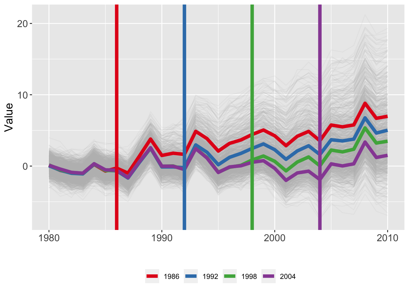

Figure 4.40: Average outcomes in Baker’s dataset

Let’s estimate an event-study regression on this data:

\[\begin{align*} y_{i,t} & = \mu_i + \delta_t + \sum_{k\neq -1}\beta_k1\{D^k_{i,t}=k\} + \epsilon_{i,t}, \end{align*}\]

where $D^k_{i,t}$ measures the time to treatment. In practice, we bin together all the treated observations that are treated more than 5 time periods ahead and, in a separate dummy, all the observations that have been treated more than 5 time periods before. Let’s run the regression (note that Andrew Baker uses the felm function of the lfe package instead of the feols function of the fixest package that we have prefentially used):

# variables we will use
keepvars <- c("`rel_year_-5`",  "`rel_year_-4`",  "`rel_year_-3`",  "`rel_year_-2`",
               "rel_year_0", "rel_year_1", "rel_year_2", "rel_year_3", "rel_year_4", "rel_year_5")

# make dummy columns
data.baker <- data.baker %>% 
    # make dummies
    mutate(rel_year = year - cohort_year) %>% 
    dummy_cols(select_columns = "rel_year") %>% 
    # generate pre and post dummies
     mutate(Pre = ifelse(rel_year < -5, 1, 0),
            Post = ifelse(rel_year > 5, 1, 0))
  
# estimate the model
mod <- felm(dep_var ~ Pre + `rel_year_-5` + `rel_year_-4` + `rel_year_-3` + `rel_year_-2` + 
                `rel_year_0` + `rel_year_1` + `rel_year_2` + `rel_year_3` + `rel_year_4` + 
                `rel_year_5` + Post | unit + year | 0 | state, data = data.baker, exactDOF = TRUE)
  
# grab the obs we need
DIDBakerEstimTWFEBinned <- broom::tidy(mod) %>% 
    filter(term %in% keepvars) %>% 
    mutate(t = c(-5:-2, 0:5)) %>% 
    select(t, estimate,std.error) %>%
    bind_rows(tibble(t = -1, estimate = 0, std.error = 0)) %>% 
    mutate(true_tau = ifelse(t >= 0, (t + 1)*.3, 0))

Let us now plot the results estimates:

  ggplot(aes(x = t, y = estimate),data=DIDBakerEstimTWFEBinned) + 
  geom_linerange(aes(ymin = estimate-1.96*std.error, ymax = estimate+1.96*std.error), color = 'darkgrey', size = 2) + 
  geom_point(color = 'blue', size = 4) + 
  geom_line(aes(x = t, y = true_tau), color = 'red', linetype = "dashed", size = 2) + 
  geom_hline(yintercept = 0, linetype = "dashed") + 
  scale_x_continuous(breaks = -5:5) + 
  labs(x = "Relative Time", y = "Estimate") + 
  theme(axis.title = element_text(size = 14),
        axis.text = element_text(size = 12))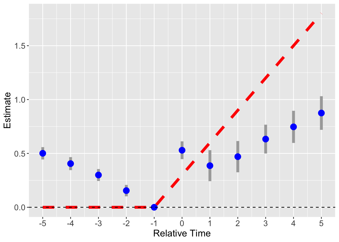

Figure 4.41: Binned Two Way Fixed Effects estimator in Baker’s dataset

The true estimates (in red) appear to have been severely misestimated by the TWFE binned estimator. The pre-trends, which are parallel in the generated data, appear to be affected by a downward slope with the Two Way Fixed Effects estimator. The treatment effects do not increase continuously over time, as they should, and they are most of the time biased downwards.

There are two main problems with the event-study model estimated with the TWFE estimator on the data plotted in Figure 4.40:

The binned treatment groups, especially the post treatment group, that regroups all observations that have been in the treatment for more than 5 years, does not move after once has entered it. It thus serves as a control group for the more recently treated, which generates a reverse DID estimator, which is biased when treatment effects grow over time.
Post 2003, all groups are treated and there thus are no untreated observations to serve as a control group, except for the post treatment binned group. This exacerbates the first problem.

The cures for this issues seem to:

Never bin observations post-treatment, so that they are never used in a reverse DID design.
Never include time periods without any control group in the data.

Let’s see what happens when we stop binning our post-treatment observations, we drop all treatment years for which there are no controls and we replace the time-to-treatment indicator by a constant for the never treated group (so that it is not used to build the time to treatment indicators, but only as a control group, to estimate the time fixed effects).

data.baker <- data.baker %>%
    filter(year <= 2003) %>% 
    mutate(cohort_year = ifelse(cohort_year == 2004, 0, cohort_year)) %>% 
    # make relative year indicator
    mutate(rel_year = year - cohort_year)
  
# get the minimum relative year - we need this to reindex
min_year <- min(data.baker %>% filter(cohort_year != 0) %>% pull(rel_year))
  
# reindex the relative years
data.baker <- data.baker %>% 
    mutate(rel_year = rel_year - min_year) %>% 
    dummy_cols(select_columns = "rel_year")
  
# make regression formula 
indics <- paste("rel_year", (1:max(data.baker %>% filter(cohort_year != 0) %>% pull(rel_year)))[-(-1 - min_year)], sep = "_", collapse = " + ")
keepvars <- paste("rel_year", c(-5:-2, 0:5) - min_year, sep = "_")  
formula <- as.formula(paste("dep_var ~", indics, "| unit + year | 0 | state"))
  
# run mod
mod <- felm(formula, data = data.baker, exactDOF = TRUE)
  
# grab the obs we need
DIDBakerEstimTWFECorrect <- broom::tidy(mod) %>% 
    filter(term %in% keepvars) %>% 
    mutate(t = c(-5:-2, 0:5)) %>% 
    select(t, estimate, std.error) %>%
    bind_rows(tibble(t = -1, estimate = 0, std.error=0)) %>% 
    mutate(true_tau = ifelse(t >= 0, (t + 1)*.3, 0))

Let us now plot the data:

ggplot(aes(x = t, y = estimate),data=DIDBakerEstimTWFECorrect) + 
  geom_linerange(aes(ymin = estimate-1.96*std.error, ymax = estimate+1.96*std.error), color = 'darkgrey', size = 2) + 
  geom_point(color = 'blue', size = 4) + 
  geom_line(aes(x = t, y = true_tau), color = 'red', linetype = "dashed", size = 2) + 
  geom_hline(yintercept = 0, linetype = "dashed") + 
  scale_x_continuous(breaks = -5:5) + 
  labs(x = "Relative Time", y = "Estimate") + 
  theme(axis.title = element_text(size = 14),
        axis.text = element_text(size = 12))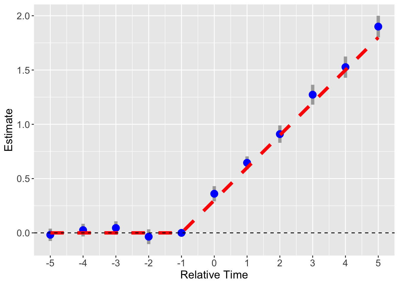

Figure 4.42: Corrected Two Way Fixed Effects estimator in Baker’s dataset

So, in general, Sun and Abraham bias seems to come from a misleading binning of treated observations post treatment and the absence of a never treated group. Let us check whether this would generate weird results for the Two-Way Fixed Effects estimator in our dataset as well.

Example 4.52 Let us check whether binning the post-treatment observations together (let’s say the last two) generates bias for the event study estimator in our original dataset. We distinguish between an estimator using the data from the always takers and an estimator not using these observations.

# generating the binned indicator
data <- data %>%
          mutate(
            TimeToTreatmentBinned = if_else(TimeToTreatment<=0,TimeToTreatment,1)
          )

# event study regression
# without the always treated
reg.TWFE.event.study.binned.No1 <- feols(y ~ i(TimeToTreatmentBinned,ref=c(-99,-1)) | id + time, data=filter(data,Ds>1))
# with the always treated
reg.TWFE.event.study.binned.1 <- feols(y ~ i(TimeToTreatmentBinned,ref=c(-99,-1)) | id + time, data=data)

Let us now plot the event study estimates obtained using Two Way Fixed Effects-based methods with binned data:

# putting results into a dataframe
resultsTWFEEventStudyBinned <- as.data.frame(rbind(cbind(reg.TWFE.event.study.binned.No1$coefficients[1:4],reg.TWFE.event.study.binned.No1$se[1:4]),
                                                  cbind(reg.TWFE.event.study.binned.1$coefficients[1:4],reg.TWFE.event.study.binned.1$se[1:4])))
colnames(resultsTWFEEventStudyBinned) <- c('Coef','Se')
# adding the time to treatment variable
resultsTWFEEventStudyBinned <- resultsTWFEEventStudyBinned %>%
                              mutate(
                                TimeToTreatment = rep(c(-3,-2,0,1),2)
                              )
# adding the reference periods
resultsTWFEEventStudyBinned <- rbind(resultsTWFEEventStudyBinned,c(0,0,-1))
resultsTWFEEventStudyBinned <- rbind(resultsTWFEEventStudyBinned,c(0,0,-1))

# adding the method dummy
resultsTWFEEventStudyBinned <- resultsTWFEEventStudyBinned %>%
                              mutate(
                                Method = c(rep("Without Always Treated",4),rep("With Always Treated",4),c("Without Always Treated","With Always Treated"))
                              )

#plot
ggplot(resultsTWFEEventStudyBinned,aes(x=TimeToTreatment,y=Coef,color=Method,linetype=Method))+
    geom_line() +
    geom_pointrange(aes(ymin=Coef-1.96*Se,ymax=Coef+1.96*Se)) +
    ylab("DID estimate") +
    xlab("Time relative to treatment") +
    scale_x_continuous(breaks=c(-3,-2,-1,0,1,2)) +
    expand_limits(y=0) +
    theme_bw()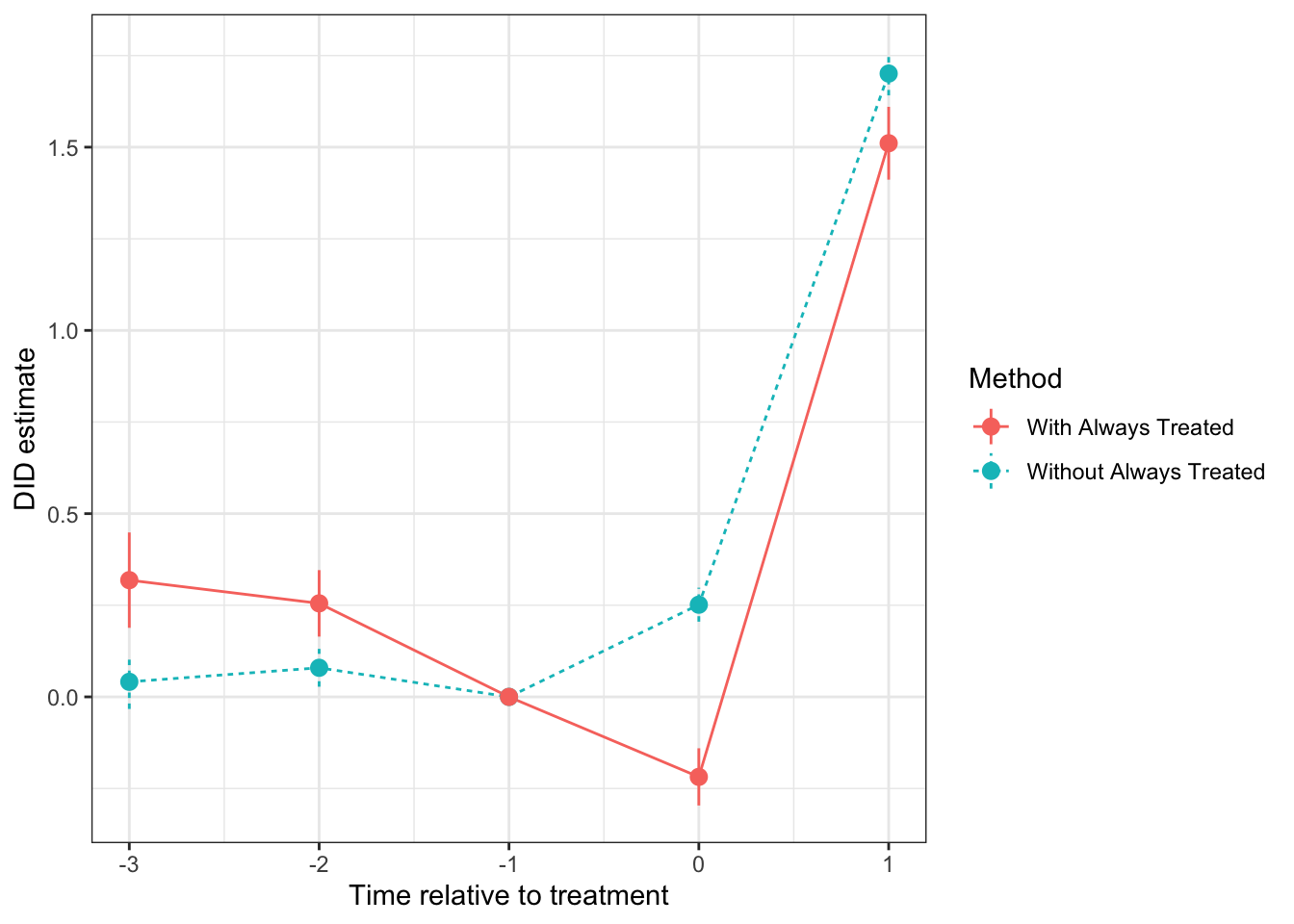

$DID estimates around the treatment date estimated using the Binned TWFE estimator (reference period $\tau'=1$)$

Figure 4.43: DID estimates around the treatment date estimated using the Binned TWFE estimator (reference period $\tau'=1$)

Figure 4.43 confirms the analysis based on Andrew Baker’s data presented in Figure 4.41. Binning the data post-treatment severely biases the event study graph estimated using a Two-Way Fixed Effects estimator, especially if one keeps the always treated observations in the dataset.

4.3.3.2.10 Summary

Let us regroup all the event study estimates and all the aggregated estimates of the TT together in order to compare them with the true estimator. Let us start with the event study estimates first.

4.3.3.2.10.1 Event study estimates

# let us first combine all the estimators together
DID.event.study.all <- rbind(
                          DID.tau %>% filter(d=="Aggregate") %>% select(tau,ATT.tau) %>% mutate(Method="Weighted DID",Se=0) %>% rename(TimeToTreatment=tau,Coef=ATT.tau),
                          disaggregate.SA %>% filter(Group=="Aggregate") %>% select(TimeToTreatment,Coef,Se) %>% mutate(Method="Sun & Abraham"),
                          DID.CSA %>% filter(Group=="Aggregate") %>% select(TimeToTreatment,Coef,Se) %>% mutate(Method="Callaway & SantAnna"),
                          DID.dCdH %>% mutate(Method="de Chaisemartin & d'Haultfoeuille"),
                          DID.BJS %>% select(TimeToTreatment,Coef,Se) %>% mutate(Method="Borusyak, Jaravel & Speiss"),
                          resultsGardnerEventStudy %>% select(TimeToTreatment,Coef,Se) %>% mutate(Method="Gardner"),
                          resultsStackedDIDEventStudy %>% select(TimeToTreatment,Coef,Se) %>% mutate(Method="Stacked DID"),
                          resultsTWFEEventStudy %>% select(TimeToTreatment,Coef,Se) %>% mutate(Method="TWFE")
                        ) 

# Let us now add the true value of the treatment effect in the sample.
# it is not easy to estimate 
# we are going to use variable weights and the meriod -1 as reference (taking its treatment effect our of all treatment effect estimates)
DID.truth <- data %>%
              mutate(
                alpha = if_else(D==1,y1-y0,0)
              ) %>%
              filter(Group>1) %>%
              group_by(TimeToTreatment) %>%
              summarize(
                Coef=if_else(TimeToTreatment>=0,mean(alpha),0)
              ) %>%
              mutate(
                Method="Truth",
                Se=0
              ) %>%
              filter(TimeToTreatment<3) 

# regrouping
DID.event.study.all <- rbind(DID.event.study.all,DID.truth) %>%
                        mutate(
                          Method=factor(Method,levels=c("Truth","Weighted DID","Sun & Abraham","Callaway & SantAnna","de Chaisemartin & d'Haultfoeuille","Borusyak, Jaravel & Speiss","Gardner","Stacked DID","TWFE"))
                        )

Let us now plot the data:

# plot
ggplot(DID.event.study.all,aes(x=TimeToTreatment,y=Coef,colour=Method,linetype=Method,shape=Method))+
    geom_line() +
    geom_pointrange(aes(ymin=Coef-1.96*Se,ymax=Coef+1.96*Se)) +
    ylab("DID estimate") +
    xlab("Time relative to treatment") +
    scale_x_continuous(breaks=c(-3,-2,-1,0,1,2)) +
    expand_limits(y=0) +
    scale_colour_discrete(name="Treatment\ngroup")+
    scale_linetype_discrete(name="Treatment\ngroup")+
    scale_shape_discrete(name="Treatment\ngroup")+
    theme_bw()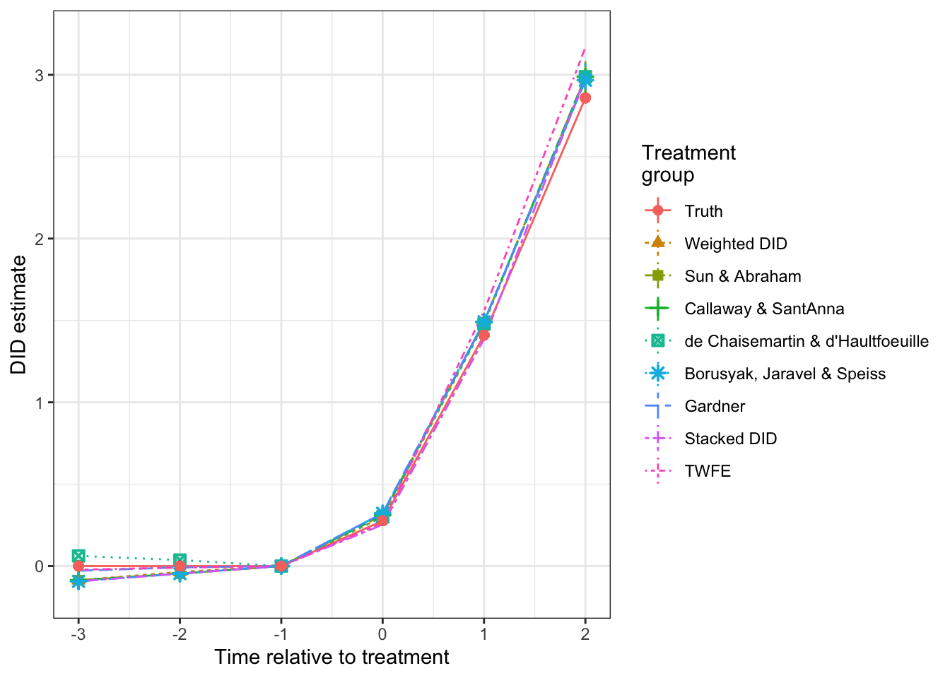

$Event study estimates around the treatment date with various methods (reference period $\tau'=1$)$

Figure 4.44: Event study estimates around the treatment date with various methods (reference period $\tau'=1$)

Note that all estimators are pretty similar. There is a dip 3 periods before treatment for some estimators. It is actually a true dip due to time varying selection bias at the first period which is embedded in the model.

Remark. Another approach to compare all estimators would be to use directly the did2s package. The command event_study uses almost all the commands already presented and integrates them into one unique analysis. Let’s see how this works.

# modifying the name of the control group variable to 0
data <- data %>%
          mutate(
            Ds=if_else(Ds==99,0,Ds)
          )
# regression
reg.event.study.all <- event_study(data=filter(data,Ds!=1),yname = "y", idname="id", tname = "time",gname="Ds")

# modifying the name of the control group variable back to 99
data <- data %>%
          mutate(
            Ds=if_else(Ds==0,99,Ds)
          )

Let’s now plot the results. It is made super easy by the command plot_event_study but we could also use the same ggplot command that we have used so far.

# using the plot_event_study command (not super nice, so not shown)
# plot_event_study(reg.event.study.all,seperate = F)

# preparing data 
reg.event.study.all <- reg.event.study.all %>%
                        mutate(
                          estimator=factor(estimator,levels=c("Sun and Abraham (2020)","Callaway and Sant'Anna (2020)","Borusyak, Jaravel, Spiess (2021)","Gardner (2021)","TWFE","Roth and Sant'Anna (2021)"))
                        ) %>%
                        rename(
                          Method=estimator,
                          Coef=estimate,
                          Se=std.error,
                          TimeToTreatment=term
                        )

# using classical ggplot
ggplot(reg.event.study.all,aes(x=TimeToTreatment,y=Coef,group=Method,color=Method))+
    geom_line() +
    geom_pointrange(aes(ymin=Coef-1.96*Se,ymax=Coef+1.96*Se)) +
    ylab("DID estimate") +
    xlab("Time relative to treatment") +
    scale_x_continuous(breaks=c(-3,-2,-1,0,1,2)) +
    expand_limits(y=0) +
    theme_bw()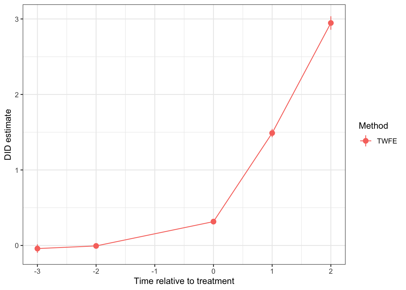

$DID estimates around the treatment date estimated using various procedures (reference period $\tau'=1$)$

Figure 4.45: DID estimates around the treatment date estimated using various procedures (reference period $\tau'=1$)

There is a problem here, let’s hope we can find a way to solve it.

4.3.3.2.10.2 Aggregate Treatment on the Treated Estimates

Let us now see what happens to the average effect of the treatment on the treated.

# let us first combine all the estimators together
DID.TT.all <- DID.event.study.all <- rbind(
                          data.frame(Coef=c(ATT.equal),Se=c(0)) %>% mutate(Method="Weighted DID Equal",Se=0),
                          data.frame(Coef=c(ATT.varying),Se=c(0)) %>% mutate(Method="Weighted DID Varying",Se=0),
                          as.data.frame(ATT.agg.SA) %>% rename(Coef=Estimate,Se=colnames(ATT.agg.SA)[[2]]) %>% select(Coef,Se) %>% mutate(Method="Sun & Abraham"),
                          as.data.frame(ATT.agg.CSA[1:2]) %>% rename(Coef=overall.att,Se=overall.se) %>% mutate(Method="Callaway & SantAnna"),
                          data.frame(Coef=c(reg.dCdH$effect),Se=c(0)) %>% mutate(Method="de Chaisemartin & d'Haultfoeuille"),
                          reg.BJS.Agg[2:3] %>% rename(Coef=estimate,Se=std.error) %>% mutate(Method="Borusyak, Jaravel & Speiss"),
                          data.frame(Coef=coef(reg.Gardner)[[1]],Se=se(reg.Gardner)[[1]]) %>% mutate(Method="Gardner"),
                          data.frame(Coef=coef(reg.stacked.aggregate)[[1]],Se=se(reg.stacked.aggregate)[[1]]) %>% mutate(Method="Stacked DID"),
                          data.frame(Coef=reg.TWFE.aggregate$coefficients[[1]],Se=reg.TWFE.aggregate$se[[1]]) %>% mutate(Method="TWFE")
                        ) 

# Let us now add the true value of the treatment effect in the sample.
ATT.truth <- data %>%
              filter(Group>1,D==1) %>%
              mutate(
                 alpha = y1-y0
               ) %>%
              summarize(
                Coef=mean(alpha)
              ) %>%
              mutate(
                Method="Truth",
                Se=0
              ) 

# regrouping
DID.TT.all <- rbind(DID.TT.all,ATT.truth) %>%
                        mutate(
                          Method=factor(Method,levels=c("Truth","Weighted DID Equal","Weighted DID Varying","Sun & Abraham","Callaway & SantAnna","de Chaisemartin & d'Haultfoeuille","Borusyak, Jaravel & Speiss","Gardner","Stacked DID","TWFE"))
                        )

Let us now plot the results:

# plot
ggplot(DID.TT.all,aes(x=Method,y=Coef))+
    geom_pointrange(aes(ymin=Coef-1.96*Se,ymax=Coef+1.96*Se)) +
    ylab("DID estimate") +
    xlab("Method") +
    expand_limits(y=0) +
    coord_flip() +
    theme_bw()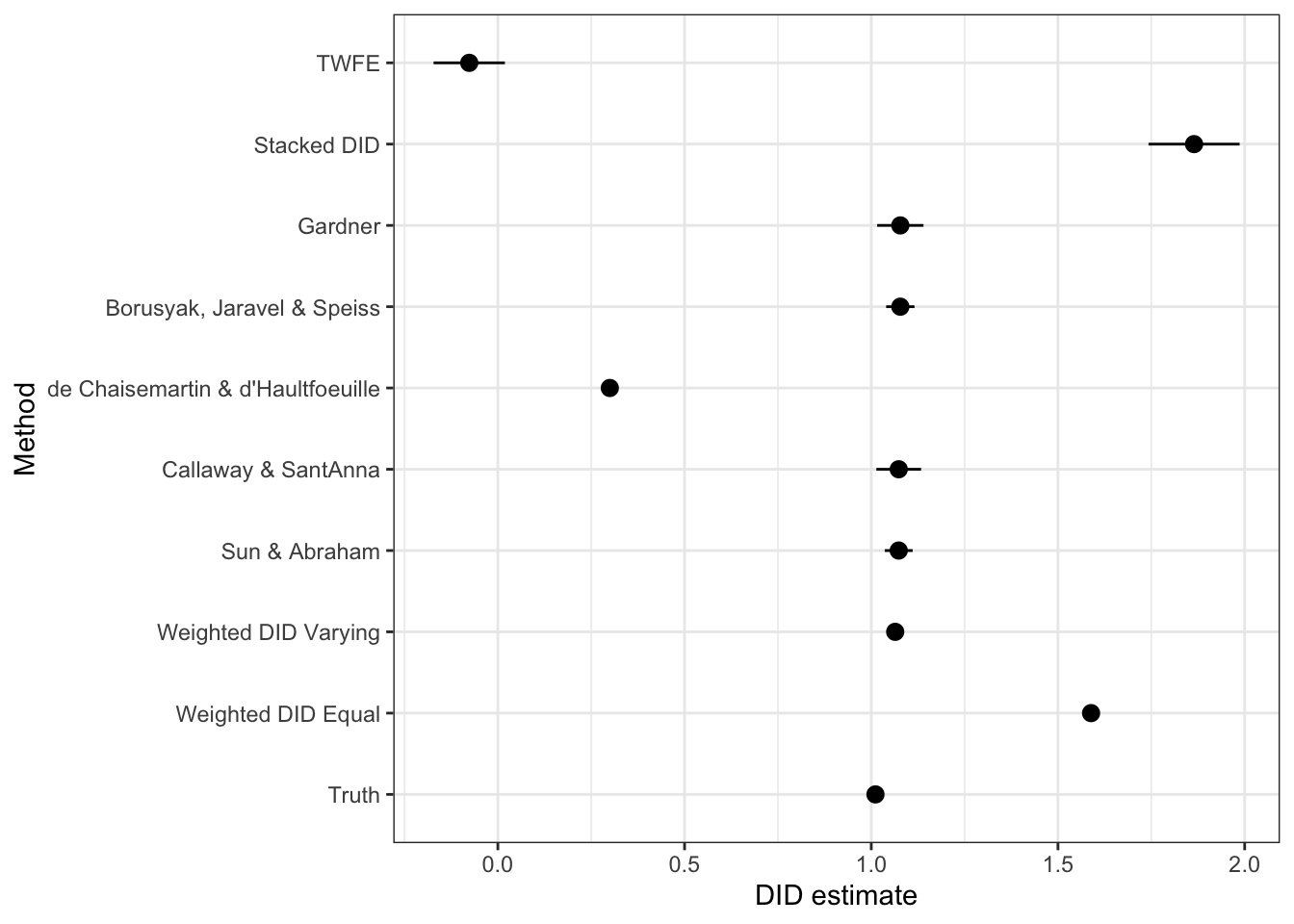

$Average treatment effect on the treated estimates with various methods (reference period $\tau'=1$)$

Figure 4.46: Average treatment effect on the treated estimates with various methods (reference period $\tau'=1$)

Figure 4.46 shows that the true effect of the treatment in the sample (with weights proportional to actual exposure to the treatment) is correctly estimated by the Weighted DID estimator using weights varying with exposure, but also by the correct estimators of Sun and Abraham, Callaway and Sant’Anna, Borusyak, Jaravel and Speiss and Gardner. The Two-Way fixed Effect estimator finds a negative treatment effect whereas all treatment effects are positive. The Stacked DID estimator finds too large a treatment effect, probably because it gives too much weight to later treatment periods. The de Chaisemartin and d’Haultfoeuille estimator used here only aims at estimating the effect of the treatment in the first time period, for which it is consistent.

Remark. Several open questions remain after this section. They are mostly cosmetic since thay are questions about properties of the Two-Way Fixed Effects estimator, and thus do not affect the properties of the correct estimators that we have studied:

Does the Two Way Fixed Effect estimator recover a correct treatment effect (that is only with positive weights) when the equivalent to Assumption 4.19 holds?
Does the event-study Two Way Fixed Effect estimator recover the correct dynamics of treatment effects when there is no binning of the treated observations past some date, and there is a never treated group that is used to estimate the time fixed effects? Our example in Section 4.3.3.2.9.2 seems to suggest that it is so, while the slightly different results of that estimator with respect to the correct ones in the summary of results above seems to suggest otherwise. An example where the event-study Two Way Fixed Effect estimator fails but these conditions hold would be very useful to understand the scope of Theorem 4.23 better.
Does the gain in efficiency obtained by the imputation estimator is still present when combining all the DID estimates from all the possible comparison groups, as in the weigthed DID estimator we have proposed?

4.3.3.3 Estimation of sampling noise

We now need to derive the asymptotic distribution of our estimators in a staggered DID design. We are going to do that for the Sun and Abraham estimator, which is the simplest estimator that is estimated by OLS, Within, LSDV, First Difference or faster TWFE estimators and extends the simple DID estimators to staggered designs. There are two sets of parameters for which we might want to know their distribution: the parameter specific to each treated group and relative time to treatment $\hat\beta^{SA}_{d,\tau}$ and the aggregated treatment effect $\hat\Delta^{Y}_{TT}(k)$ for some set of weights $w^k(d,d',\tau,\tau')$. Let’s look at these parameters in turn.

4.3.3.3.1 Estimation of sampling noise for the effect of the treatment on each group and at each time period

We can estimate the $\hat\beta^{SA}_{d,\tau}$ with either repeated cross section data or panel data. Let us start with studying what happens with repeated cross sections before moving to panel data.

4.3.3.3.1.1 Estimation of sampling noise for the effect of the treatment on each group and at each time period with repeated cross sections

With repeated cross sections, we can only use the OLS DID estimator of the Sun and Abraham model. The following theorem derives its distribution:

Theorem 4.24 (Asymptotic Distribution of Sun and Abraham Estimator in Repeated Cross Sections) Under Assumptions 4.12, 4.13, 4.14, 4.17 and 2.3, and with repeated cross sections of total size $N$, we have:

\[\begin{align*} \sqrt{N}(\hat\beta^{SA}_{d,\tau}-\beta^{SA}_{d,\tau}) & \stackrel{d}{\rightarrow} \mathcal{N}\left(0,\frac{1}{p^{d,\tau}} \left[\frac{\var{Y^0_{i,d-1}|D_i=\infty}}{(1-p^{d,\tau}_D)(1-p^{d,\tau}_A)} +\frac{\var{Y^0_{i,d-1}|D_i=d}}{p^{d,\tau}_D(1-p^{d,\tau}_A)}\right.\right. \\ & \phantom{\stackrel{d}{\rightarrow}\mathcal{N}\left(0,\frac{1}{p^{d,\tau}}\right.}\left.\left. +\frac{\var{Y^0_{i,d+\tau}|D_i=\infty}}{(1-p^{d,\tau}_D)p^{d,\tau}_A} +\frac{\var{Y^1_{i,d+\tau}|D_i=\infty}}{p^{d,\tau}_Dp^{d,\tau}_A} \right]\right) \end{align*}\]

where $p^{d,\tau}=\Pr((D_i=d\cup D_i=\infty)\cap(T_i=d-1\cup T_i=d+\tau))$, $p^{d,\tau}_D=\Pr(D_i=d|(D_i=d\cup D_i=\infty)\cap(T_i=d-1\cup T_i=d+\tau))$ and $p^{d,\tau}_A=\Pr(T_i=d+\tau|(D_i=d\cup D_i=\infty)\cap(T_i=d-1\cup T_i=d+\tau))$.

Proof. See Section A.3.5.

Remark. Note that Theorem 4.24 is very close to Theorem 4.12. The only difference is the additional $p^{d,\tau}$ term which adjusts the sample size by the actual number of observations used in the estimation of $\hat\beta^{SA}_{d,\tau}$.

4.3.3.3.1.2 Estimation of sampling noise for the effect of the treatment on each group and at each time period with panel data

With panel data, we can estimate $\hat\beta^{SA}_{d,\tau}$ using various sets of estimators: the OLS DID model, the within transformation of the Sun and Abraham model with individual dummies, the Least Squares Dummy Variables model estimated by OLS, the First Difference model and the enhanced estimators (Alternating Projections and Likelihood Concentration). Theorem 4.20 implies that all these estiamtors are similar and identical to the individual DID estimators. We can thus use Theorem 4.11 in order to provide a CLT-based estimate the sampling noise of the Sun and Abraham estimator of the individual treatment effects in panel data. The following theorem derives its distribution:

Theorem 4.25 (Asymptotic Distribution of Sun and Abraham Estimator in Panel Data) Under Assumptions 4.12, 4.13, 4.14, 4.15 and 4.16, and with panel data with $N$ units observed over $T$ periods, we have:

\[\begin{align*} \sqrt{N}(\hat\beta^{SA}_{d,\tau}-\beta^{SA}_{d,\tau}) & \stackrel{d}{\rightarrow} \mathcal{N}\left(0,\frac{1}{p^{d,\infty}}\left(\frac{\var{Y_{i,d+\tau}^1-Y_{i,d-1}^0|D_i=d}}{p^{d,\infty}_D}+\frac{\var{Y_{i,d+\infty}^0-Y_{i,d-1}^0|D_i=\infty}}{1-p^{d,\infty}_D}\right)\right), \end{align*}\]

where $p^{d,\infty}=\Pr(D_i=d\cup D_i=\infty)$ and $p^{d,\infty}_D=\Pr(D_i=d|D_i=d\cup D_i=\infty)$.

Proof. See Section A.3.7.

4.3.3.3.2 Estimation of sampling noise for aggregate treatment effects

The key now is to derive the distribution of the event study parameters and of the average treatment effect on the treated. We are going to use the Delta Method in order to do so, but that requires determining the covariance matrix of the $\hat\beta_{d,\tau}^{SA}$ parameters. Under Assumption 4.15 for panel data or 4.17 in repeated cross sections, most of the $\hat\beta_{d,\tau}^{SA}$ parameters are independent from each other, except for the ones which make use of the same parts of the data.

4.3.3.3.2.1 Estimation of sampling noise for aggregate treatment effects with repeated cross sections

The following theorem derives the asymptotic distribution of the aggregated treatment on the treated parameter based on the individual DID estimates stemming from Sun and Abraham’s estimator, in repeated cross sections.

Theorem 4.26 (Asymptotic Distribution of Treatment of the Treated Estimated Using Sun and Abraham Estimator in Repeated Cross Sections) Under Assumptions 4.12, 4.13, 4.14, 4.17 and 2.3, and with repeated cross sections of total size $N$, we have:

\[\begin{align*} \sqrt{N}(\hat\Delta^{Y}_{TT_{SA}}(k)-\Delta^{Y}_{TT_{SA}}(k)) & \stackrel{d}{\rightarrow} \mathcal{N}\left(0,\sum_d\sum_{\tau}V(\hat\beta^{SA}_{d,\tau})(w^k(d,d-1,\tau,\infty))^2 \right.\\ & \phantom{\stackrel{d}{\rightarrow}}\left.+\sum_{d}\sum_{d'}\sum_{\tau}\sum_{\tau'\neq\tau} \text{Cov}(\hat\beta^{SA}_{d,\tau},\hat\beta^{SA}_{d',\tau'})w^k(d,d-1,\tau,\infty)w^k(d',d'-1,\tau',\infty)\right), \end{align*}\]

where:

\[\begin{align*} V(\hat\beta^{SA}_{d,\tau}) & =\frac{1}{p^{d,\tau}}\left[\frac{\var{Y^0_{i,d-1}|D_i=\infty}}{(1-p^{d,\tau}_D)(1-p^{d,\tau}_A)} +\frac{\var{Y^0_{i,d-1}|D_i=d}}{p^{d,\tau}_D(1-p^{d,\tau}_A)}\right. \\ & \phantom{=} \left.+\frac{\var{Y^0_{i,d+\tau}|D_i=\infty}}{(1-p^{d,\tau}_D)p^{d,\tau}_A} +\frac{\var{Y^1_{i,d+\tau}|D_i=\infty}}{p^{d,\tau}_Dp^{d,\tau}_A}\right]\\ \text{Cov}(\hat\beta^{SA}_{d,\tau},\hat\beta^{SA}_{d',\tau'}) & = \frac{p^{d,\tau,d',\tau'}p_{d-1}^{d,\tau,d',\tau'}}{p^{d,\tau}p^{d',\tau'}} \left[\frac{\var{Y^0_{i,d-1}|D_i=\infty}(1-p_D^{d,\tau,d',\tau'})}{(1-p_A^{d,\tau})(1-p_A^{d',\tau'})(1-p_D^{d,\tau})(1-p_D^{d',\tau'})} \right.\\ & \phantom{=\frac{p^{d,\tau,d',\tau'}p_{d-1}^{d,\tau,d',\tau'}}{p^{d,\tau}p^{d',\tau'}}}\left. +\frac{\var{Y^0_{i,d-1}|D_i=d}p_D^{d,\tau,d',\tau'}}{(1-p_A^{d,\tau})(1-p_A^{d',\tau'})p_D^{d,\tau}p_D^{d',\tau'}}\right] \text{ when } d=d'\\ & = \frac{p^{d,\tau,d',\tau'}p_{d+\tau}^{d,\tau,d',\tau'}\var{Y^0_{i,d+\tau}|D_i=\infty}(1-p_D^{d,\tau,d',\tau'})}{p^{d,\tau}p^{d',\tau'}p_A^{d,\tau}p_A^{d',\tau'}(1-p_D^{d,\tau})(1-p_D^{d',\tau'})}\text{ when } d+\tau=d'+\tau' \\ & = -\frac{p^{d,\tau,d',\tau'}p_{d-1}^{d,\tau,d',\tau'}\var{Y^0_{i,d-1}|D_i=\infty}(1-p_D^{d,\tau,d',\tau'})}{p^{d,\tau}p^{d',\tau'}(1-p_A^{d,\tau})p_A^{d',\tau'}(1-p_D^{d,\tau})(1-p_D^{d',\tau'})} \text{ when } d-1=d'+\tau'\\ & = -\frac{p^{d,\tau,d',\tau'}p_{d'-1}^{d,\tau,d',\tau'}\var{Y^0_{i,d'-1}|D_i=\infty}(1-p_D^{d,\tau,d',\tau'})}{p^{d,\tau}p^{d',\tau'}p_A^{d,\tau}(1-p_A^{d',\tau'})(1-p_D^{d,\tau})(1-p_D^{d',\tau'})} \text{ when } d+\tau=d'-1\\ & = 0 \text{ otherwise}. \end{align*}\]

with $p^{d,\tau}=\Pr((D_i=d\cup D_i=\infty)\cap(T_i=d-1\cup T_i=d+\tau))$, $p^{d,\tau}_D=\Pr(D_i=d|(D_i=d\cup D_i=\infty)\cap(T_i=d-1\cup T_i=d+\tau))$, $p^{d,\tau}_A=\Pr(T_i=d+\tau|(D_i=d\cup D_i=\infty)\cap(T_i=d-1\cup T_i=d+\tau))$, $p^{d,\tau,d',\tau'}=\Pr(D_j^{d',\tau'}D_j^{d,\tau}=1)$, $p_{d+\tau}^{d,\tau,d',\tau'}=\Pr(T_j=d+\tau|D_j^{d',\tau'}D_j^{d,\tau}=1)$ and $p_D^{d,\tau,d',\tau'}=\Pr(D_j^{d'}=1\cup D_j^{d}=1|D_j^{d',\tau'}D_j^{d,\tau}=1)$.

Proof. See Section A.3.6.

Remark. Note that the covariance terms in Theorem 4.26 make a lot of sense. First, the proportions used to normalize the variance terms correspond exactly to the proportion of observations in the relevant groups. Second, the signs of the covariances are consistent with common sense. When $d=d'$, the individual components $\hat\beta^{SA}_{d,\tau}$ and $\hat\beta^{SA}_{d',\tau'}$ estimate the impact for the same treatment group. They thus share their baseline means (both for the treated and control group observed at period $d-1$). As a consequence, they are positively correlated. When $d+\tau=d'+\tau'$, both groups share the same post-treatment period, and thus use the same observations from the control group to build the After period, thereby generating a positive correlation again. When $d-1=d'+\tau'$ or $d'-1=d+\tau$, both estimators share the same group of observations from the control group. One uses them as a reference period, while the other uses the same observations as the after treatment period. As a consequence, the estimators are negatively correlated in that case.

4.3.3.3.2.2 Estimation of sampling noise for aggregate treatment effects with panel data

Finally, we need to determine the asymptotic distribution of the aggregate average treatment effect on the treated $\Delta^Y_{TT}(k)$ in panel data. Panel data are a very different animal from repeated cross sections in that we follow the same individuals over time. We thus need to be extra careful on what we assume on the correlation of the outcomes of each individual over time. In this section, we are going to rule out any autocorrelation between error terms in levels. We will relax this assumption later.

We encode our main assumption on autocorrelation of outcomes over time as follows:

Hypothesis 4.28 (i.i.d. sampling in panel data) We assume that potential outcomes are geenrated as follows:

\[\begin{align*} Y^0_{i,t} & = \mu_i + \delta_t + U^0_{i,t}\\ Y^1_{i,t} & = \mu_i + \delta_t + \bar{\alpha} +\eta_{i,t} + U^0_{i,t}, \end{align*}\]

with $\esp{U^0_{i,t}}=\esp{\eta_{i,t}}=0$, $\forall t$, $\esp{U^0_{i,t}|D_i}=0$, $\forall t$ and:

\[\begin{align*} \forall i,j\leq N\text{, }\forall t,t'\leq T\text{, with either }i\neq j \text{ or } t\neq t' & (U^0_{i,t},\eta_{i,t},D_i)\Ind(U^0_{j,t'},\eta_{j,t'},D_j),\\ & (U^0_{i,t},\eta_{i,t},D_i)\&(U^0_{j,t'},\eta_{j,t'},D_j)\sim F_{U^0,\eta,D} . \end{align*}\]

Remark. Assumption 4.28 is restrictive. For example, it prevents error terms to be correlated over time for each unit $i$, which requires $\rho=0$ in our toy model. It also requires that individual treatment effects are not autocorrelated over time, which for example requires that $\theta_d=0$ in our model and that $\eta_{i,t}$ is not autocorrelated over time. It means that treatment effects cannot be correlated with fixed effects, a huge assumption, and that agents with high treatment effects at one period are not more likely to have high treatment effects the next period. These assumptions are obviously too strong. We will see how to relax them in Chapter 9.

Remark. Note that Assumption 4.28 implies Assumption 4.14. The proof is left as an exercise.

Theorem 4.27 (Asymptotic Distribution of Treatment of the Treated Estimated Using Sun and Abraham Estimator in Panel Data) Under Assumptions 4.12, 4.13, 4.14, 4.28 and 4.16, and with panel data containing a total of $N$ units observed over $T$ time periods, we have:

\[\begin{align*} \sqrt{N}(\hat\Delta^{Y}_{TT_{SA}}(k)-\Delta^{Y}_{TT_{SA}}(k)) & \stackrel{d}{\rightarrow} \mathcal{N}\left(0,\sum_d\sum_{\tau}V_P(\hat\beta^{SA}_{d,\tau})(w^k(d,d-1,\tau,\infty))^2\right.\\ & \phantom{\stackrel{d}{\rightarrow}}\left.+\sum_{d}\sum_{d'}\sum_{\tau}\sum_{\tau'\neq\tau} \text{Cov}_P(\hat\beta^{SA}_{d,\tau},\hat\beta^{SA}_{d',\tau'})w^k(d,d-1,\tau,\infty)w^k(d',d'-1,\tau',\infty)\right), \end{align*}\]

where:

\[\begin{align*} V_P(\hat\beta^{SA}_{d,\tau}) & =\frac{1}{p^{d,\infty}}\left(\frac{\var{Y_{i,d+\tau}^1-Y_{i,d-1}^0|D_i=d}}{p^{d,\infty}_D}+\frac{\var{Y_{i,d+\tau}^0-Y_{i,d-1}^0|D_i=\infty}}{1-p^{d,\infty}_D}\right)\\ \text{Cov}_P(\hat\beta^{SA}_{d,\tau},\hat\beta^{SA}_{d',\tau'}) & = \frac{1}{p^{d,\infty}}\left[\frac{\var{U^0_{i,d-1}|D_i=\infty}}{1-p^{d,\infty}_D}+\frac{\var{U^0_{i,d-1}|D_i=d}}{p^{d,\infty}_D}\right] \text{ when } d=d'\\ & = \frac{1}{p^{d',\infty}}\frac{\var{U^0_{i,d'+\tau'}|D_i=\infty}}{1-p^{d',\infty}_D} \text{ when } d+\tau=d'+\tau' \\ & = -\frac{1}{p^{d',\infty}}\frac{\var{U^0_{i,d'+\tau'}|D_i=\infty}}{1-p^{d',\infty}_D} \text{ when } d-1=d'+\tau' \\ & = -\frac{1}{p^{d,\infty}}\frac{\var{U^0_{i,d+\tau}|D_i=\infty}}{1-p^{d,\infty}_D} \text{ when } d+\tau=d'-1\\ & = 0 \text{ otherwise}, \end{align*}\]

with $p^{d,\infty}=\Pr(D_i=d\cup D_i=\infty)$ and $p^{d,\infty}_D=\Pr(D_i=d|D_i=d\cup D_i=\infty)$.

Proof. See Section A.3.8.

Remark. The result in Theorem 4.27 makes intuitive sense. Under Assumption 4.28, the only source of correlation between individual treatment effects $\hat\beta^{SA}_{d,\tau}$ and $\hat\beta^{SA}_{d',\tau'}$ is when they share part of the data that yields to their estimation. When $d=d'$, they share the same reference period for both the treated and the untreated groups. When $d+\tau=d'+\tau'$, they share the same end period for the untreated group. It means that in both of these cases, the two estimators are positively correlated. When $d-1=d'+\tau'$ or when $d+\tau=d'-1$, the reference period of one serves as the ending period for the other, both for the untreated group. In these two cases, the two estimators are negatively correlated.

Remark. Note also that the result in Theorem 4.27 suggests that, in some cases, the treatment on the treated parameter is going to be more precise than the individual level estimates. Let’s assume for simplicity one treatment group, $\frac{T}{2}$ treatment periods, the same variance for all individual level estimates, the same weigths for combining them in the ATT ($\frac{2}{T}$) and no correlation between each individual estimator, then we have $V_P(\hat\Delta^{Y}_{TT_{SA}}(k))=\frac{2}{T}V_P(\hat\beta^{SA})$, which is smaller than $V_P(\hat\beta^{SA})$ as soon as $T\geq 3$. Intuitively, under the assumptions in this remark, each individual estimate is an independent estimate of the same parameter, and thus, according to the CLT, precision increases with the square root of the number of additional observations, which is proportional to $\sqrt{\frac{2}{T}}$. Under more general conditions, this simple relationship might not hold. It might be the case for example that some treatment effects might be less precisely estimated than others, and thus that the precision of the resulting average treatment effect might be intermediate between the precision of the two individual estimates. The existence of covariance terms between the individual treatment estimates might also increase (or decrease) the eventual precision of the average treatment effect estimate.

4.3.3.3.3 Estimation of sampling noise in practice

Until now, we have looked at sampling noise in a theoretical way. Let’s see in practice how to estimate sampling noise in a staggered DID design in practice. There are several ways to estimate sampling noise for the Sunn and Abraham estimator that we have studied in detail. We could either use the plug-in formulas we have derived in Theorems 4.24, 4.25, 4.26 and 4.27. We could also use the heteroskedasticity-robust standard errors that the fixest package spits out when using feols with the sunab option. We could also use only the $2\times 2$ DID estimators with a first difference estimator using OLS and heteroskedasticity-robust standard errors. We could also use the stacked First Difference estimator that we have use in the proof of Theorem 4.20 (we know it is identical to the Sun and Abraham estimator) and use a heteroskedasticity-robust covariance matrix estimator.

For now, we are going to compare the estimates of sampling noise stemming from $2\times 2$ DID estimators and the stacked First Difference estimator to the ones stemming from the fixest implementation of Sun and Abraham estimator, and to the true level of sampling noise stemming from Monte Carlo simulations. We are also going to compare the estimates of sampling noise for the TT parameter using the fixest implementation of Sun and Abraham estimator and the stacked First Difference estimator and compare them to the Monte Carlo estimates. Let’s go.

Example 4.53 Let’s see how $2\times 2$ DID estimators, the stacked First Difference estimator and the fixest implementation of Sun and Abraham estimator perform in our example.

In order to do so, we are first going to write a function implementing our $2\times 2$ DID estimators automatically.

# function estimating 2x2 DID and heteroskedasticity-robust standard error with within and first difference estimators
# StaggeredDID22 is a function that takes as inputs:
# y: name of outcome variable (character)
# D: name of treatment group variable (character)
# d: treatment group defined by date of entry into the treatment
# dprime: comparison group
# tau: number of periods after treatment date at which we estimate the effect of the treatment
# tauprime: number of periods before the treatment date that we use a baseline period (defaults to one)
# t: time indicator (character)
# i: individual unit indicator (character)
# data: dataset containing the outcomes and treatments and time and unit indicators
StaggeredDID22 <- function(tau,d,y,D,dprime,tauprime=1,t,i,data){
  # taking out the irrelevant groups and time periods and generating a useful treatment variable
  data.DID <- data %>%
            filter(!!sym(D) == d | !!sym(D) == dprime) %>% 
            filter(!!sym(t) == d+tau | !!sym(t)==d-tauprime) %>%
            mutate(
              Dit = if_else(!!sym(D) == d & !!sym(t) == d+tau,1,0),
              time = case_when(
                        !!sym(t) == d+tau ~ 1,
                        !!sym(t) == d-tauprime ~ 0,
                        TRUE ~ 9999
              )
            )
  # running the within estimator (fixest)
  # regression formula for the within estimator
  DID.form <- as.formula(paste(paste(y,paste("Dit",t,sep="+"),sep="~"),i,sep="|"))
  reg.W.fixest <- feols(DID.form,vcov='HC1',data = data.DID)
  # regression for the first difference estimator
  data.DID <- data.DID %>%
                pivot_wider(id_cols=!!sym(i),names_from=time,values_from=c('Dit',y),names_sep='_') %>%
                mutate(
                  DeltaY = !!sym(paste(y,1,sep='_'))-!!sym(paste(y,0,sep='_')),
                  DeltaD = !!sym(paste('Dit',1,sep='_'))-!!sym(paste('Dit',0,sep='_'))
                )
  DID.FD.form <- as.formula(paste(paste("DeltaY","DeltaD",sep="~"),1,sep="|"))
  reg.FD.fixest <- feols(DID.FD.form,vcov='HC1',data = data.DID)
  # result vector
  DID.est.W.fixest <- c(d,dprime,tau,tauprime,coef(reg.W.fixest)[[1]],sqrt(vcov(reg.W.fixest)[[1,1]]),coef(reg.FD.fixest)[[2]],sqrt(vcov(reg.FD.fixest)[[2,2]]))
  names(DID.est.W.fixest) <- c("d","dprime","tau","tauprime","WithinEst","WithinSe","FDEst","FDSe")
  return(DID.est.W.fixest)
}
#test <- StaggeredDID22(tau=1,d=2,y='y',D='Ds',dprime=99,tauprime=1,t="time",i="id",data=data)

Let’s now write a function implementing the stacked First Difference estimator automatically.

# function estimating 2x2 DID and heteroskedasticity-robust standard error and covariance matrix with stacked first difference
# StackedDIDFD is a function that takes as inputs:
# y: name of outcome variable (character)
# D: name of treatment group variable (character)
# dprime: comparison group
# tauprime: number of periods before the treatment date that we use a baseline period (defaults to one)
# t: time indicator (character)
# i: individual unit indicator (character)
# Leung: whether we use a Leung-robust covariance matrix for time
# data: dataset containing the outcomes and treatments and time and unit indicators
StackedDIDFD <- function(y,D,dprime.ref,tauprime.ref=1,t,i,Leung="None",data){
  # levels of the treatment (without never treated)
  d <- data %>% mutate(test = as.factor(!!sym(D))) %>% pull(test) %>% levels(.) %>% as.character(.) %>% as.numeric(.) 
  d <- d[d!=dprime.ref]
  d <- d[order(d)]
  # list of possible treatment periods for each treatment group
  # first, list of time periods
  time <- data %>% mutate(test = as.factor(!!sym(t))) %>% pull(test) %>% levels(.) %>% as.numeric(.) 
  time <- time[order(time)]
  # dataset of all treatment groups and all time periods
  d.expand <- unlist(lapply(d,rep,length(time)))
  time.expand <- rep(time,length(d))
  data.structure <- data.frame(d=d.expand,time=time.expand) %>%
    # time in relative periods for each d
    mutate(
      TimeToTreatment = time-d
    ) %>%
  # detection of treatment groups without any reference period
    mutate(
      ReferencePeriod = case_when(
        TimeToTreatment == -1 ~ 1,
        TRUE ~ 0
      )
    ) 
  # Treatment groups without reference period (for whom estimation is impossible)
  Groups.impossible <- data.structure %>%
                        group_by(d) %>%
                        summarize(
                          MaxReferencePeriod = max(ReferencePeriod)
                        ) %>%
                        filter(MaxReferencePeriod==0) %>%
                        pull(d) %>%
                        unique(.) 
  # Treatment groups with a reference period (for whom estimation is possible)
  Groups.possible <- data.structure %>% 
                      group_by(d) %>%
                      mutate(
                        MaxReferencePeriod = max(ReferencePeriod)
                      ) %>%
                      filter(MaxReferencePeriod==1) %>%
                      pull(d) %>%
                      unique(.)
  # data for which estimation if feasible
  data.structure <- data.structure %>% 
                      group_by(d) %>%
                      mutate(
                        MaxReferencePeriod = max(ReferencePeriod)
                      ) %>%
                      filter(MaxReferencePeriod==1) %>%
                      select(-MaxReferencePeriod)
  # Adding one line for each time we need the reference period
  data.ref <- data.structure %>%
                mutate(
                  ReferencePeriodName = d-as.numeric(tauprime.ref)
                ) %>%
                filter(ReferencePeriod==0) %>%
                mutate(
                  ReferencePeriod=1
                ) %>%
                rename(
                  TimeToTreatmentStar=TimeToTreatment,
                  timestar=time 
                ) 
  data.structure <- data.structure %>%
                      mutate(
                        ReferencePeriodName = d-as.numeric(tauprime.ref)
                      ) %>%
                      left_join(data.ref,by=c('d','ReferencePeriod','ReferencePeriodName')) %>%
                      mutate(
                        TargetPeriod=case_when(
                          !is.na(timestar) ~ timestar,
                          is.na(timestar) ~ time,
                          TRUE~999999
                        ),
                        TargetTimeToTreatment=case_when(
                          !is.na(TimeToTreatmentStar) ~ TimeToTreatmentStar,
                          is.na(TimeToTreatmentStar) ~ TimeToTreatment,
                          TRUE~999999
                        )
                      ) %>%
                      select(-timestar,-TimeToTreatmentStar) 
  
  # building the stacked DID dataset
  data.structure <- data.structure %>%
                      mutate(
                        dstar = d
                      ) %>%
                      rename(
                        TimeToTreatmentStructure = TimeToTreatment
                      )
  
  data.structure.control <- data.structure %>%
                      mutate(
                        dstar = as.numeric(dprime.ref)
                      )
  data.structure <- rbind(data.structure,data.structure.control)
  Stacked.DID.Data <- data.structure %>%
                        left_join(data,by=c('time'=t,'dstar'=D)) %>% 
                        select(id,time,d,dstar,TimeToTreatmentStructure,ReferencePeriod,ReferencePeriodName,TargetPeriod,TargetTimeToTreatment,!!sym(y)) %>%
                        arrange(id,d,TargetPeriod,ReferencePeriod) %>%
                        pivot_wider(id_cols=c('id','d','TargetPeriod','TargetTimeToTreatment','dstar'),names_from="ReferencePeriod",names_prefix = y,values_from=c(y)) %>%
                        mutate(
                          DeltaY = !!sym(paste(y,'0',sep=""))-!!sym(paste(y,'1',sep="")),
                          D = case_when(
                            dstar == as.numeric(dprime.ref) ~ 0,
                            TRUE ~ 1
                          ),
                          D = factor(D,levels=c('0','1')),
                          Ddtau = paste(d,TargetTimeToTreatment,sep=',')
                        ) %>%
                        arrange(Ddtau,D,id) %>%
                        ungroup(.)
   
  # generating the covariates matrix (using the recipes package)
   DeltaX <- recipe(~ Ddtau+D,data=Stacked.DID.Data)  %>% 
    step_dummy(Ddtau,one_hot = TRUE) %>% 
    step_dummy(D) %>% 
    step_interact(terms=~starts_with("Ddtau"):D_X1) %>% 
    prep(training=Stacked.DID.Data) %>% 
    bake(new_data=NULL)  %>%
    select(-D_X1) 
   # order the variables and make DeltaX a matrix
   DeltaX <- DeltaX %>%
    relocate(colnames(DeltaX)[order(colnames(DeltaX))]) %>%
    as.matrix(.) # make it Sparse
  # generating the outcomes matrix
   DeltaY <- Stacked.DID.Data %>%
              select(DeltaY) %>%
              as.matrix(.)
  # inverting the covariance matrix
  DeltaXDeltaXm1 <- solve(t(DeltaX)%*%DeltaX)
  # Esimating the coefficients of the stacked DID model using OLS
  Stacked.DID.OLS.Theta <- DeltaXDeltaXm1%*%t(DeltaX)%*%DeltaY
  # recovering the coefficients
  Coefs.Stacked.DID.FD <- as.data.frame(Stacked.DID.OLS.Theta) 
  
  Coefs.Stacked.DID.FD <- as.data.frame(Stacked.DID.OLS.Theta) %>%
                            mutate(
                              Groups=rownames(Coefs.Stacked.DID.FD),
                              Beta0 = str_split_fixed(Groups,'x',n=2)[,2],
                              Beta1 = str_split_fixed(Groups,'x',n=2)[,1],
                              Beta2 = str_split_fixed(Beta1,'X',n=2)[,2],
                              minus.tau = str_detect(Beta2,'\\.\\.'),
                              d = str_split_fixed(Beta2,'\\.',n=2)[,1],
                              tau = str_split_fixed(Beta2,'\\.',n=2)[,2],
                              tau = str_extract(tau,".?\\d*"),
                              tau = case_when(
                                minus.tau==TRUE ~ str_split_fixed(tau,'\\.',n=2)[,2],
                                TRUE~tau
                              ),
                              tau = case_when(
                                minus.tau ~ -as.numeric(tau),
                                TRUE ~ as.numeric(tau)
                              ),
                              Ddtau = paste(d,tau,sep=',')
                            ) %>%
                            rename(TE = DeltaY) %>%
                            filter(Beta0!="") %>%
                            select(-contains("Beta"),-Groups,-minus.tau) %>%
                            relocate(TE,.after="tau") %>%
                            relocate(Ddtau) 
  
  # estimating standard errors for the BetaSAdtau parameters using Theorem 4.25
  VarBetaSA.d.tau <- Stacked.DID.Data %>%
                        group_by(Ddtau,D) %>%
                        summarize(
                          VarDeltaYdtau = var(DeltaY),
                          Nd = n() 
                        ) %>%
                        mutate(VarDeltaYdtau.N = VarDeltaYdtau/Nd) %>%
                        group_by(Ddtau) %>%
                        summarize(
                          VarDeltaYdtau.N = sum(VarDeltaYdtau.N)
                        ) %>%
                       mutate(
                          d = as.numeric(str_split_fixed(Ddtau,pattern=",",n=2)[,1]),
                          tau = as.numeric(str_split_fixed(Ddtau,pattern=",",n=2)[,2])
                       ) %>%
                      arrange(d,tau)

  # estimating covariances between treatment effect parameters using Theorem 4.27
  # First, I need estimates of the Us, which come out of the feols estimator
  # I can only run it on a data set with only observations used for estimation
  data.res <- data %>% 
                filter(!(!!sym(D) %in% Groups.impossible))
  reg.DID.SA <- feols(as.formula(paste(paste(y,paste('sunab(',paste(D,t,sep=','),')',sep=''),sep='~'),paste(i,t,sep='+'),sep='|')),vcov='HC1',data=data.res)
  data.res$residuals <- reg.DID.SA$residuals
  # Form all possible combinations of d,tau and d',tau'
  Ddtau.dprime.tauprime <- t(combn(VarBetaSA.d.tau$Ddtau,2)) %>%
                            as.data.frame(.) %>%
                            rename(
                              Ddtau = V1,
                              D.dprime.tauprime = V2
                            ) %>%
                            # generate d, tau, dprime and tauprime
                            mutate(
                              d = as.numeric(str_split_fixed(Ddtau,pattern=",",n=2)[,1]),
                              tau = as.numeric(str_split_fixed(Ddtau,pattern=",",n=2)[,2]),
                              dprime = as.numeric(str_split_fixed(D.dprime.tauprime,pattern=",",n=2)[,1]),
                              tauprime = as.numeric(str_split_fixed(D.dprime.tauprime,pattern=",",n=2)[,2])
                            ) %>%
                            # generate the cases of Theorem 4.27, with both the time period at which the variance has to be computed and for which group
                            mutate(
                              Cases = case_when(
                                          d==dprime ~ 1,
                                          d+tau==dprime+tauprime ~ 2,
                                          d-tauprime.ref==dprime+tauprime ~ 3,
                                          d+tau==dprime-tauprime.ref ~ 4,
                                          TRUE ~ 0
                                        ),
                              Period = case_when(
                                          Cases==1 ~ d-tauprime.ref,
                                          Cases==2 ~ d+tau,
                                          Cases==3 ~ d-tauprime.ref,
                                          Cases==4 ~ dprime-tauprime.ref,
                                          TRUE ~ 0
                                        ),
                              Group = case_when(
                                        Cases==1 ~ "All",
                                        Cases >1 ~ "0",
                                        TRUE ~ "None"
                                      )
                            )
  # Generating the variance terms
  Var.residuals <- data.res %>%
                        group_by(!!sym(t),!!sym(D)) %>%
                        summarize(
                          VarUdt = var(residuals),
                          Ndt = n() 
                        ) %>%
                        mutate(VarUdt.N = VarUdt/Ndt) %>%
                        ungroup(.) %>%
                        select(-VarUdt,-Ndt) %>%
                        rename(d=!!sym(D))
  # Separating the variance terms for the treated, the controls and summing them as well
  # treated
  Var.residuals.1 <- Var.residuals %>%
                        filter(d!=dprime.ref) %>%
                        mutate(Group="All")
  # untreated
  Var.residuals.0 <- Var.residuals %>%
                        filter(d==dprime.ref) %>%
                        mutate(Group="0")
  # creating the covariances
  # joining the variances of the untreated for cases 2 to 4
  Ddtau.dprime.tauprime <- Ddtau.dprime.tauprime %>%
                            left_join(Var.residuals.0 %>% select(-d),by=c('Period'=t,'Group'='Group')) %>%
                            rename(VarUdt.N.0=VarUdt.N)
  # preparing data of non treated for joining in case 1
  Var.residuals.0 <- Var.residuals.0 %>%
                        mutate(Group="All")
  Ddtau.dprime.tauprime <- Ddtau.dprime.tauprime %>%
                            left_join(Var.residuals.0 %>% select(-d),by=c('Period'=t,'Group'='Group')) %>%
                            rename(VarUdt.N.0.All=VarUdt.N) %>%
                            left_join(Var.residuals.1,by=c('Period'=t,'Group'='Group','d'='d')) %>%
                            rename(VarUdt.N.1.All=VarUdt.N) %>%
                            mutate(
                              Cov.dtau.dprime.tauprime = case_when(
                                                            Cases==1 ~ VarUdt.N.0.All+VarUdt.N.1.All,
                                                            Cases==2 ~ VarUdt.N.0,
                                                            Cases==3 ~ -VarUdt.N.0,
                                                            Cases==4 ~ -VarUdt.N.0,
                                                            TRUE ~ 0
                                                          )
                            ) %>%
                            select(-contains('VarUdt.N'))

  if (Leung=="Temporal"){
    # estimating the residuals
    Stacked.DID.OLS.res <- DeltaY-DeltaX%*%Stacked.DID.OLS.Theta
    # estimating the Leung covariance matrix
    # product of the matrix of covariates times the residuals
    M <- DeltaX*as.numeric(Stacked.DID.OLS.res) # only use it in teh computation
    # generating a matrix of "connexions" between observations: under the absence of autocorrelation assumption, identifies the observations that are used several times
    # make it sparse using the Matrix package
    # for that: generate a unique identifier for each line in the dataset and match it back to find all the lines that correspond
    Stacked.DID.Data <- Stacked.DID.Data %>%
                         arrange(Ddtau,D,id) %>%
                         mutate(
                           column.id = 1:nrow(Stacked.DID.Data)
                         ) %>%
                         relocate(column.id)
    Merged.Stacked.DID.Data <- Stacked.DID.Data %>%
                               left_join(Stacked.DID.Data,by='id')
    G <- Matrix::sparseMatrix(Merged.Stacked.DID.Data$column.id.x,Merged.Stacked.DID.Data$column.id.y,dims = c(nrow(Stacked.DID.Data),nrow(Stacked.DID.Data))) 
    #SparseM::image(G)
    Vcov.Stacked.DID.OLS.Theta.Leung <- DeltaXDeltaXm1%*%t(DeltaX*as.numeric(Stacked.DID.OLS.res))%*%G%*%(DeltaX*as.numeric(Stacked.DID.OLS.res))%*%DeltaXDeltaXm1
    # recovering vcov matrix of the coeffcients (the 2x2 DID coefficients are the even elements of the coefficient vector)                        
    Vcov.Coefs.Stacked.DID.FD.Leung <- as.matrix(Vcov.Stacked.DID.OLS.Theta.Leung[c(FALSE,TRUE),c(FALSE,TRUE)])
  }
  # recovering stadnard error of the coefficients
  Coefs.Stacked.DID.FD <- Coefs.Stacked.DID.FD %>%
                            left_join(VarBetaSA.d.tau %>% select(Ddtau,VarDeltaYdtau.N),by='Ddtau') %>%
                            mutate(
                              SeTE = sqrt(VarDeltaYdtau.N)
                            ) %>%
                            select(-VarDeltaYdtau.N)
  # adding reference periods
  # groups used for estimation
  d.ref <- Groups.possible
  DID.ref <- data.frame(d=d.ref,tau=-1,TE=0,SeTE=0) %>%
                mutate(Ddtau = paste(d,tau,sep=','))
  Coefs.Stacked.DID.FD <- rbind(Coefs.Stacked.DID.FD,DID.ref) %>%
                        arrange(d,tau)

  # generating the covariance matrix
  columns.cov.matrix <- data.frame(Ddtau=Coefs.Stacked.DID.FD$Ddtau,Ddtau.id=1:length(Coefs.Stacked.DID.FD$Ddtau))
  Ddtau.dprime.tauprime <- Ddtau.dprime.tauprime %>%
                            left_join(columns.cov.matrix,by=c('Ddtau'='Ddtau'))   %>%
                            left_join(columns.cov.matrix,by=c('D.dprime.tauprime'='Ddtau'))
  Vcov.Coefs.Stacked.DID.FD <- Matrix::sparseMatrix(i=Ddtau.dprime.tauprime$Ddtau.id.x,j=Ddtau.dprime.tauprime$Ddtau.id.y,x=Ddtau.dprime.tauprime$Cov.dtau.dprime.tauprime,dims=c(length(Coefs.Stacked.DID.FD$Ddtau),length(Coefs.Stacked.DID.FD$Ddtau))) 
  # symmetrize matrix and add diagonal
  Vcov.Coefs.Stacked.DID.FD <- as.matrix(Vcov.Coefs.Stacked.DID.FD+t(Vcov.Coefs.Stacked.DID.FD)+diag(Coefs.Stacked.DID.FD$SeTE^2))
  colnames(Vcov.Coefs.Stacked.DID.FD) <- Coefs.Stacked.DID.FD$Ddtau
  rownames(Vcov.Coefs.Stacked.DID.FD) <- Coefs.Stacked.DID.FD$Ddtau
  
  # estimating ATT (varying weights) and its standard error
  # estimating the weights: each treated period has a weight, which depends on its proportion in the total number of treated observations
  # keeping all observations that are part of the treated groups used for estimation
  ATT.DID.weights <- DID.ref %>%
                      select(d) %>%
                      left_join(data,by=c('d'=D)) %>%
                      rename(Period=!!sym(t)) %>%
                      group_by(d,Period) %>%
                      summarize(
                        Ntreated = n()
                      )%>%
                      ungroup(.)   %>%
                      # keep only treated periods
                      mutate(
                        TimeToTreatment = Period-d,
                        Ntreated = if_else(TimeToTreatment < 0,0,as.numeric(Ntreated)), 
                        N = sum(Ntreated),
                        weights=Ntreated/N,
                        TimeToTreatment=!!sym(t)-d
                      ) %>%
                      arrange(d,Period)
  # ATT
  ATT <- t(ATT.DID.weights[,"weights"])%*%Coefs.Stacked.DID.FD[,"TE"]
  ATTSe <- sqrt(t(ATT.DID.weights[,"weights"])%*%Vcov.Coefs.Stacked.DID.FD%*%as.matrix(ATT.DID.weights[,"weights"]))
  
  # results
  result <- list(Coefs.Stacked.DID.FD,Vcov.Coefs.Stacked.DID.FD,ATT,ATTSe)
  names(result) <- c("BetaSA","VcovBetaSA","ATT","ATTSe")
  
  # add Leung estimates if needed
  if (Leung=="Temporal"){
    # ATT
    ATTSe.Leung <- sqrt(t(ATT.DID.weights %>% filter(weights>0) %>% select("weights"))%*%Vcov.Coefs.Stacked.DID.FD.Leung[str_detect(colnames(Vcov.Coefs.Stacked.DID.FD.Leung),'\\.\\.',negate=TRUE),str_detect(colnames(Vcov.Coefs.Stacked.DID.FD.Leung),'\\.\\.',negate=TRUE)]%*%as.matrix(ATT.DID.weights %>% filter(weights>0) %>% select("weights")))
    # results
    result <- list(Coefs.Stacked.DID.FD,Vcov.Coefs.Stacked.DID.FD,ATT,ATTSe,ATTSe.Leung,Vcov.Coefs.Stacked.DID.FD.Leung)
    names(result) <- c("BetaSA","VcovBetaSA","ATT","ATTSe","ATTSeLeung","VcovBetaSALeung")
  }
  return(result)
}

# test 
test.stacked.DID.FD <- StackedDIDFD(y='y',D='Ds',dprime=99,tauprime=1,t="time",i="id",Leung='Temporal',data=data)

We now are going to write a function taking a set of parameter values and a sample size and spitting out $2\times 2$ DID estimates with their standard errors and the fixest implementation of Sun and Abraham estimator, both for individual level estimates and for the aggregate treatment effect.

# function generating a sample with N sample size and spitting out DID estimates (both event study and TT, with both Sunab and 2x2 DID)
# seed: seed setting the PRNG
# N: number of units in the panel
# T: number of periods in the panel (cannot be different from 4 in this instance ;)
# param: basic parameters
Outcome.Sample.DID <- function(seed,N,T=4,param){
  # simulating a sample
  set.seed(seed)
  cov.eta.omega <- matrix(c(param["sigma2eta"],param["rhoetaomega"]*sqrt(param["sigma2eta"]*param["sigma2omega"]),param["rhoetaomega"]*sqrt(param["sigma2eta"]*param["sigma2omega"]),param["sigma2omega"]),ncol=2,nrow=2)
  data <- as.data.frame(rmvnorm(N*T,c(0,0),cov.eta.omega))
  colnames(data) <- c('eta','omega')
  # time and individual identifiers
  data$time <- c(rep(1,N),rep(2,N),rep(3,N),rep(4,N))
  data$id <- rep((1:N),T)
  # unit fixed effects
  data$mu <- rep(rnorm(N,param["barmu"],sqrt(param["sigma2mu"])),T)
  # time fixed effects
  data$delta <- c(rep(param["delta1"],N),rep(param["delta2"],N),rep(param["delta3"],N),rep(param["delta4"],N))
  data$baralphat <- c(rep(param["baralpha1"],N),rep(param["baralpha2"],N),rep(param["baralpha3"],N),rep(param["baralpha4"],N))
  
  # building autocorrelated error terms
  data$epsilon <- rnorm(N*T,0,sqrt(param["sigma2epsilon"]))
  data$U[1:N] <- rnorm(N,0,sqrt(param["sigma2U"]))
  data$U[(N+1):(2*N)] <- param["rho"]*data$U[1:N] + data$epsilon[(N+1):(2*N)]
  data$U[(2*N+1):(3*N)] <- param["rho"]*data$U[(N+1):(2*N)] + data$epsilon[(2*N+1):(3*N)]
  data$U[(3*N+1):(T*N)] <- param["rho"]*data$U[(2*N+1):(3*N)] + data$epsilon[(3*N+1):(T*N)]
  # potential outcomes in the absence of the treatment
  data$y0 <- data$mu + data$delta + data$U 
  data$Y0 <- exp(data$y0)
  # treatment timing
  # error term
  data$V <- param["gamma"]*(data$mu-param["barmu"])+data$omega
  # treatment group, with 99 for the never treated instead of infinity
  Ds <- if_else(data$y0[1:N]+param["xi1"]+data$V[1:N]<=log(param["barY"]),1,
                if_else(data$y0[1:N]+param["xi2"]+data$V[1:N]<=log(param["barY"]),2,
                        if_else(data$y0[1:N]+param["xi3"]+data$V[1:N]<=log(param["barY"]),3,
                                if_else(data$y0[1:N]+param["xi4"]+data$V[1:N]<=log(param["barY"]),4,99))))
  data$Ds <- rep(Ds,T)
  # Treatment status
  data$D <- if_else(data$Ds>data$time,0,1)
  # potential outcomes with the treatment
  # effect of the treatment by group
  data$baralphatd <- if_else(data$Ds==1,param["barchi1"],
                             if_else(data$Ds==2,param["barchi2"],
                                     if_else(data$Ds==3,param["barchi3"],
                                             if_else(data$Ds==4,param["barchi4"],0))))+
                    if_else(data$Ds==1,param["kappa1"],
                             if_else(data$Ds==2,param["kappa2"],
                                     if_else(data$Ds==3,param["kappa3"],
                                             if_else(data$Ds==4,param["kappa4"],0))))*(data$t-data$Ds)*if_else(data$time>=data$Ds,1,0)
  data$y1 <- data$y0 + data$baralphat + data$baralphatd + if_else(data$Ds==1,param["theta1"],if_else(data$Ds==2,param["theta2"],if_else(data$Ds==3,param["theta3"],param["theta4"])))*data$mu + data$eta
  data$Y1 <- exp(data$y1)
  data$y <- data$y1*data$D+data$y0*(1-data$D)
  data$Y <- data$Y1*data$D+data$Y0*(1-data$D)
  
  # estimating DID model with Sun and Abraham estimator
  reg.DID.SA <- feols(y ~ sunab(Ds,time) | id + time,vcov='HC1',data=filter(data,Ds>1))
  resultsDID.SA <- data.frame(Coef=reg.DID.SA$coefficients,Se=reg.DID.SA$se,Name=names(reg.DID.SA$coefficients)) %>%
                mutate(
                  #TimeToTreatment = as.numeric(str_split_fixed(Name,'::',n=2)[,2])
                  TimeToTreatment = as.numeric(str_split_fixed(Name,':',n=4)[,3]),
                  Group = as.numeric(str_split_fixed(Name,':',n=6)[,6])
                ) %>%
                select(-Name) %>%
                relocate(TimeToTreatment,.before=Coef) %>%
                relocate(Group,.before=TimeToTreatment)
  # adding reference period
  resultsDID.SA <- rbind(resultsDID.SA,c(2,-1,0,0),c(3,-1,0,0),c(4,-1,0,0))
  # TT
  # ATT <- aggregate(reg.DID, c("ATT" = "TimeToTreatment::[^-]"))   
  ATT.SA <- aggregate(reg.DID.SA, c("ATT" = "time::[^-]"))   
  ATT.SA <- data.frame(Group="All",TimeToTreatment=99,Coef=ATT.SA[[1]],Se=ATT.SA[[2]])
  # joining results SA
  resultsDID.SA <- rbind(resultsDID.SA,ATT.SA)
  
  # estimating DID model with 2x2 FD estimators
  # generating list of final time periods specific to each treatment group
  tau <- c(0:2,-2,0:1,-3:-2,0)
  d <- c(rep(2,3),rep(3,3),rep(4,3))
  resultsDID.FD <- pmap_dfr(list(tau,d),StaggeredDID22,y='y',D='Ds',dprime=99,tauprime=1,t="time",i="id",data=data) %>%
                    select(d,tau,FDEst,FDSe) %>%
                    rename(Group=d,
                           TimeToTreatment = tau,
                           Coef=FDEst,
                           Se=FDSe) 
  # adding reference period
  resultsDID.FD <- rbind(resultsDID.FD,c(2,-1,0,0),c(3,-1,0,0),c(4,-1,0,0))
  
  # estimating the DID model with stacked FD
  results.Stacked.DID.FD.Full <- StackedDIDFD(y='y',D='Ds',dprime=99,tauprime=1,t="time",i="id",data=data) 
  results.Stacked.DID.FD <- results.Stacked.DID.FD.Full[[1]] %>%
                              rename(Group=d,
                                     TimeToTreatment = tau,
                                     Coef=TE,
                                     Se=SeTE) %>%
                              select(-Ddtau)
  # adding the ATT
  ATT.Stacked.DID.FD <- data.frame(Group="All",TimeToTreatment=99,Coef=results.Stacked.DID.FD.Full[["ATT"]],Se=results.Stacked.DID.FD.Full[["ATTSe"]]) %>%
                          rename(Se=weights)
  results.Stacked.DID.FD <- rbind(results.Stacked.DID.FD,ATT.Stacked.DID.FD)

  # joining all results
  resultsDID.SA <- resultsDID.SA %>%
                    mutate(Method = "SA")
  resultsDID.FD <- resultsDID.FD %>%
                    mutate(Method = "FD")
  results.Stacked.DID.FD <- results.Stacked.DID.FD %>%
                    mutate(Method = "StackedFD")
  resultsDID <- rbind(resultsDID.SA,resultsDID.FD,results.Stacked.DID.FD) %>%
                  relocate(Method) %>%
                  arrange(Method,Group,TimeToTreatment) %>%
                  as_tibble(.)
  # return results
  return(resultsDID)
}

# test
testDIDMC <- Outcome.Sample.DID(seed=1,N=1000,T=4,param=param)

Let us now parallelize this function.

# programming to run in parallel
# Nsim: number of simulations
# N: number of units in the panel
# T: number of periods in the panel
# param: parameters
sf.MonteCarlo.DID <- function(Nsim,N,T,param){
  sfInit(parallel=TRUE,cpus=8)
  sfLibrary(tidyverse)
  sfLibrary(fixest)
  sfLibrary(recipes)
  sfLibrary(mvtnorm)
  sfLibrary(Matrix)
  sfExport('StaggeredDID22')
  sfExport('StackedDIDFD')
  sim <- sfLapply(1:Nsim,Outcome.Sample.DID,N=N,T=T,param=param) 
  sfStop()
  # generate mean and standard error
  sim <- sim %>% 
          bind_rows(.) %>%
          group_by(TimeToTreatment,Group,Method) %>%
          summarize(
            TE = mean(Coef),
            SdTE = sd(Coef),
            MeanSeTE = mean(Se)
          ) %>%
          ungroup(.) 
  return(sim)
}
# testing
Nsim <- 10
#sf.test.MonteCarlo.DID <- sf.MonteCarlo.DID(Nsim=Nsim,N=1000,T=4,param=param)

# true simulations
Nsim <- 1000
sf.simuls.MonteCarlo.DID <- sf.MonteCarlo.DID(Nsim=Nsim,N=1000,T=4,param=param)

Let us now plot the resulting estimates. For simplicity, I center treatment effect estimates at their mean, so that we can focus on sampling noise and precision. If we did not center treatment effect estimates, variation in the size of treatment effects over time would dwarf variations in sampling noise.

# prepapring data
sf.simuls.MonteCarlo.DID <- sf.simuls.MonteCarlo.DID %>%
                                    mutate(
                                      TimeToTreatment = case_when(
                                        TimeToTreatment == "99" ~ 3,
                                        TRUE ~ TimeToTreatment
                                      ),
                                      NetTE=0
                                    ) %>%
                                    pivot_longer(cols=SdTE:MeanSeTE,names_to = "Type",values_to="SeEstim") %>%
                                    mutate(
                                      Type = case_when(
                                        Type == "MeanSeTE" ~ "Estimated",
                                        Type == "SdTE" ~ "Truth",
                                        TRUE ~ ""
                                      ),
                                      Type = factor(Type,levels=c("Truth","Estimated"))
                                    )

ggplot(sf.simuls.MonteCarlo.DID,aes(x=TimeToTreatment,y=NetTE,group=Type,color=Type,linetype=Type))+
#  geom_pointrange(aes(ymin=TE-1.96*SeEstim,ymax=TE+1.96*SeEstim),position=position_dodge(1))+
  geom_point(color='red') +
  geom_errorbar(aes(ymin=NetTE-1.96*SeEstim,ymax=NetTE+1.96*SeEstim,color=Type,group=Type,linetype=Type),position=position_dodge(0.9),width=0.3)+
  scale_x_continuous(breaks=c(-3:3)) +
  theme_bw()+
  facet_grid(Group~Method)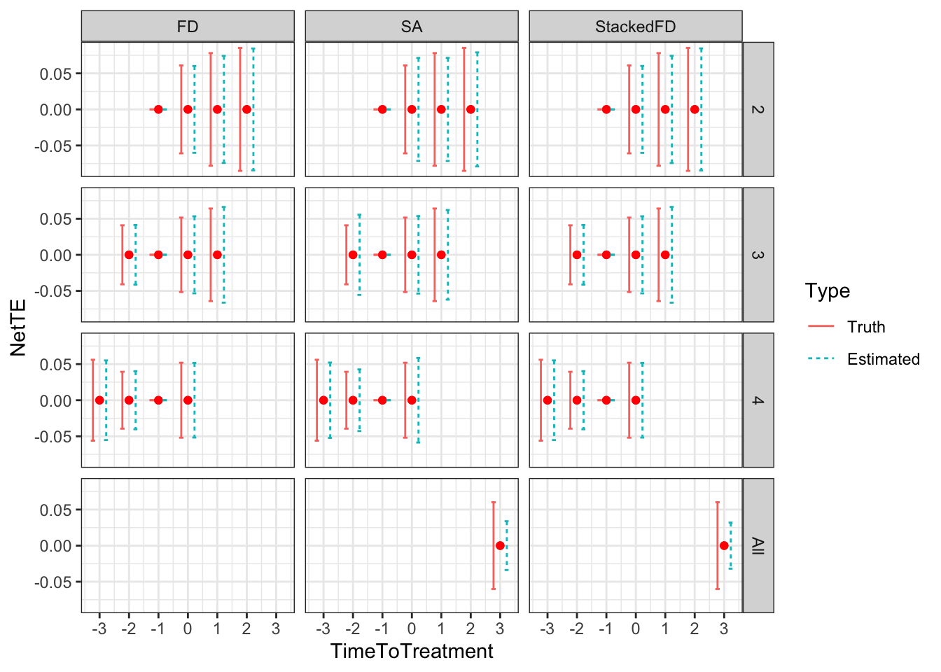

Figure 4.47: Comparison of estimates of sampling noise in staggered designs

It seems that the fixest implementation of the Sun and Abraham estimator overestimates sampling noise for some individual treatment effects (for example $d=2$ and $\tau=0$), while it underestimates sampling noise for the aggregated treatment effect. The $2\times 2$ DID estimator seems to provide much more consistent estimates of the precision of the individual level treatment effects. Both the fixest implementation of the Sun and Abraham estimator and our Stacked DID estimator seem to underestimate the sampling noise of the ATT parameter. We are going to study whether this is the case and what to do about it in Chapter 9.

4.3.4 Difference In Differences with Instrumental Variables

Sometimes, the Parallel Trends Assumption (Assumption 4.14 or Assumption 4.25 with staggered designs) does not hold. This might be because individuals select into the treatment based on unobservables correlated with the dynamics of outcomes in the absence of the treatment. One of the most famous cases in point is the dip in earnings that future participants experience before entering a Job Training Program. In that case, one might be able to reframe the Parallel Trends Assumption to hold not with respect to treatment participation, but with respect to an instrumental variable that affects participation in the treatment. In such a case, we say that we have a Difference In Differences design with Instrumental Variables or DID-IV for short. In this section, we are going to study how to identify treatment effects in this design and how to estimate them and their precision.

In DID-IV designs, a key distinction is between a strong first stage and a weak first stage. In a strong first stage, observations with a low level of the instrumental variable do not access the program, while in a weak first stage, they can. In a world of heterogeneous treatment effects, this distinction turns out to be crucial. We will first delineate identification and estimation in the case of a strong first stage, and then move on to what happens in the more complex case of a weak first stage.

4.3.4.1 DID-IV with a strong first stage

Let us first examine what is happening with DID-IV under a strong first stage. We are going to consider identification, estimation and estimation of sampling noise.

4.3.4.1.1 Identification under strong first stage DID-IV

We need some assumptions first. We are going to go back to the case where there are only two time periods, one before ($t=B$) and one after ($t=A$). We are going to keep making Assumptions 4.12 and 4.13 of absence of treatment in period $t=B$ and of absence of anticipation effects. On top of these assumptions, we are first going to assume that there is a random variable $Z_i$ taking two values ($Z_i=1$ and $Z_i=0$) such that the parallel trends assumption holds for this variable:

Hypothesis 4.29 (Parallel Trends with Instrumental Variables) We assume that the trends in the potential outcomes in the absence the treatment are the same, independent of the value of the instrumental variable:

\[\begin{align*} \esp{Y^0_{i,A}|Z_i=1} - \esp{Y^0_{i,B}|Z_i=1} & = \esp{Y^0_{i,A}|Z_i=0} - \esp{Y^0_{i,B}|Z_i=0}. \end{align*}\]

We also assume that the instrumental variables alters the probability that a unit receives the treatment:

Hypothesis 4.30 (Strong First Stage) The probability of receiving the treatment is strictly positive when $Z_i=1$ and is zero when $Z_i=0$:

\[\begin{align*} \Pr(D_i=1|Z_i=1)>\Pr(D_i=1|Z_i=0)=0. \end{align*}\]

Remark. Assumption 4.30 is really strong. Combined with Assumption 4.12, it implies that the only group which is able to receive the treament is the group with $Z_i=1$ in the After period.

Equipped with these assumptions, we can now prove the following theorem:

Theorem 4.28 (Indentification of TT with DID-IV and a Strong First Stage) Under Assumptions 4.12, 4.13, 4.29 and 4.30, TT is identified by the Wald-DID estimator:

\[\begin{align*} \Delta^Y_{WaldDID} & = \Delta^{Y_A}_{TT}, \end{align*}\]

with: \[\begin{align*} \Delta^Y_{WaldDID} & = \frac{\esp{Y_{i,A}|Z_i=1}-\esp{Y_{i,A}|Z_i=0}-(\esp{Y_{i,B}|Z_i=1}-\esp{Y_{i,B}|Z_i=0})}{\Pr(D_{i,A}=1|Z_i=1)-\Pr(D_{i,A}=1|Z_i=0)-(\Pr(D_{i,B}=1|Z_i=1)-\Pr(D_{i,B}=1|Z_i=0))}. \end{align*}\]

Proof. Under Assumption 4.29, we have:

\[\begin{align*} \esp{Y^0_{i,A}|Z_i=1} & = \esp{Y^0_{i,A}|Z_i=0} + (\esp{Y^0_{i,B}|Z_i=1}-\esp{Y^0_{i,B}|Z_i=0}) \end{align*}\]

As a consequence, the numerator of the Wald-DID estimator is:

\[\begin{align*} \esp{Y_{i,A}|Z_i=1} & -\esp{Y_{i,A}|Z_i=0}-(\esp{Y_{i,B}|Z_i=1}-\esp{Y_{i,B}|Z_i=0}) \\ & = \esp{Y_{i,A}|Z_i=1} - \esp{Y^0_{i,A}|Z_i=1} \\ & = \esp{Y^1_{i,A}|D_i=1,Z_i=1}\Pr(D_i=1|Z_i=1)+\esp{Y^0_{i,A}|D_i=0,Z_i=1}\Pr(D_i=0|Z_i=1)\\ &\phantom{=}-\esp{Y^0_{i,A}|D_i=1,Z_i=1}\Pr(D_i=1|Z_i=1)+\esp{Y^0_{i,A}|D_i=0,Z_i=1}\Pr(D_i=0|Z_i=1)\\ & = \left(\esp{Y^1_{i,A}|D_i=1,Z_i=1}-\esp{Y^0_{i,A}|D_i=1,Z_i=1}\right)\Pr(D_i=1|Z_i=1)\\ & = \Delta^{Y_A}_{TT}\Pr(D_i=1|Z_i=1), \end{align*}\]

where the last equality uses the fact that $D_i=1$ is a subset of $Z_i=1$. Using Assumption 4.30 proves that the denominator of the Wald-DID estimator is equal to $\Pr(D_i=1|Z_i=1)$, which proves the result.

Example 4.54 Let’s see how this approach works in our example. We are going to assume that there are 50 states and that the treatment is only available in half of them. This state indicator is going to be our instrumental variable. In our model, states fixed effects are going to be correlated with treatment intake (and even with $Z_i$) but $Z_i$ wil not be correlated with indiosyncratic shocks to outcomes that make people enter the treatment.

\[\begin{align*} \mu_i & = \mu^S_i + \mu^U_i + \bar{\mu} \\ \mu^S_i & \sim\mathcal{N}(0,\frac{1}{3}\sigma_{\mu}^2)\\ \mu^U_i & \sim\mathcal{N}(0,\frac{2}{3}\sigma_{\mu}^2)\\ Z _i & = \begin{cases} 1 & \text{ if } \mu^S_i\leq 0 \\ 0 & \text{ if } \mu^S_i> 0 \end{cases}\\ D_i & = \uns{y_i^B\leq\bar{y} \land Z_i=1}. \end{align*}\]

Let us first respecify the parameter vector:

param <- c(8,.5,.28,1500,0.9,0.01,0.05,0.05,0.05,0.1,0.1,7.98)
names(param) <- c("barmu","sigma2mu","sigma2U","barY","rho","theta","sigma2epsilon","sigma2eta","delta","baralpha","gamma","baryB")

Let’s simulate that dataset.

set.seed(1234)
N <-1000
param["rho"] <- 0.9
# I am going to draw a state fixed effect for 50 states with variance 1/3 of the total variance of mu
Nstates <- 50
muS <- rnorm(Nstates,0,sqrt(param["sigma2mu"]/3))
muS <- rep(muS,each=N/Nstates)
# I draw an individual fixed effect with the remaining variance
muU <- rnorm(N,0,sqrt(param["sigma2mu"]*2/3))
mu <- param["barmu"] + muS + muU 
UB <- rnorm(N,0,sqrt(param["sigma2U"]))
yB <- mu + UB 
YB <- exp(yB)
epsilon <- rnorm(N,0,sqrt(param["sigma2epsilon"]))
eta<- rnorm(N,0,sqrt(param["sigma2eta"]))
U0 <- param["rho"]*UB + epsilon
y0 <- mu +  U0 + param["delta"]
alpha <- param["baralpha"]+  param["theta"]*mu + eta
y1 <- y0+alpha
Y0 <- exp(y0)
Y1 <- exp(y1)

# Z=1 if states have lower muS than 0
Z <- ifelse(muS<=0,1,0)
Ds <- ifelse(YB<=param["barY"] & Z==1,1,0)
y <- y1*Ds+y0*(1-Ds)
Y <- Y1*Ds+Y0*(1-Ds)

Let us know look at how Assumption 4.30 holds:

# preparing the means of participants proportions
means.did.iv <- c(mean(Ds[Z==0]),mean(Ds[Z==1]),mean(y0[Z==0]),mean(y0[Z==1]),mean(y[Z==0]),mean(y[Z==1]),mean(yB[Z==0]),mean(yB[Z==1]),0,1)
means.did.iv <- matrix(means.did.iv,nrow=2,ncol=5,byrow=FALSE,dimnames=list(c('Z=0','Z=1'),c('D','y0','y','yB','Z')))
means.did.iv <- as.data.frame(means.did.iv)
# plotting the result
ggplot(means.did.iv, aes(x=as.factor(Z), y=D)) +
  geom_bar(position=position_dodge(), stat="identity", colour='black')+
  xlab('Z')+
  ylab('Pr(D=1|Z)')+
  theme_bw()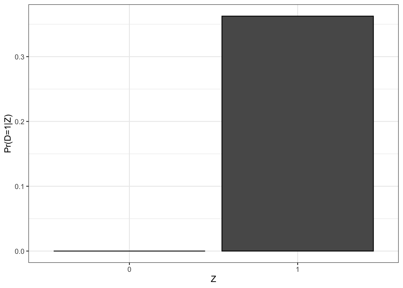

Figure 4.48: Illustration of the DID-IV assumptions: Strong First Stage

Figure 4.48 shows that no unit with $Z_i=0$ receives the treatment. We also have that $\hat{\Pr}(D_i=1|Z_i=1)=$ 0.36.

A key feature of the simulated dataset is that the parallel trends assumption does not hold for $D_i$ but it does for $Z_i$. Let’s check. We indeed have that $\hatesp{y^0_{i}|D_i=1}-\hatesp{y^B_{i}|D_i=1}=$ 0.12 and $\hatesp{y^0_{i}|D_i=0}-\hatesp{y^B_{i}|D_i=0}=$ 0.04. We also have $\hatesp{y^0_{i}|Z_i=1}-\hatesp{y^B_{i}|Z_i=1}=$ 0.06 and $\hatesp{y^0_{i}|Z_i=0}-\hatesp{y^B_{i}|Z_i=0}=$ 0.05.

The true effect of the treatment in our model is:

\[\begin{align*} \Delta^y_{TT} & = \bar{\alpha}+ \theta\esp{\mu_i|\mu_i+U_i^B\leq\bar{y} \land \mu_i^S\leq0} \end{align*}\]

To compute the expectation of a this censored normal, I use the package tmvtnorm:

The value of $\Delta^y_{TT}$ in the population is thus 0.17 and in the sample 0.17. Simple DID would not be a correct estimate of $TT$. Indeed, the value of the DID estimator in the sample is 0.24. The Wald DID estimator should be closer to the truth. In the sample, it is equal to 0.2.

4.3.4.1.2 Estimation

Estimation of the DID-IV estimator can be conducted using several approaches. Let’s review them in turn.

4.3.4.1.2.1 Using the direct Wald estimator

The most direct way to compute the DID-IV estimator in a sample is simply to compute its sample equivalent:

\[\begin{gather*} \hat{\Delta}^Y_{WaldDID}= \\ \frac{\frac{1}{\sum_{i=1}^{N}Z_i}\sum_{i=1}^{N}Y_{i,A}Z_i - \frac{1}{\sum_{i=1}^{N}(1-Z_i)}\sum_{i=1}^{N}Y_{i,A}(1-Z_i) -\left(\frac{1}{\sum_{i=1}^{N}Z_i}\sum_{i=1}^{N}Y_{i,B}Z_i - \frac{1}{\sum_{i=1}^{N}(1-Z_i)}\sum_{i=1}^{N}Y_{i,B}(1-Z_i)\right)} {\frac{1}{\sum_{i=1}^{N}Z_i}\sum_{i=1}^{N}D_{i,A}Z_i - \frac{1}{\sum_{i=1}^{N}(1-Z_i)}\sum_{i=1}^{N}D_{i,A}(1-Z_i) -\left(\frac{1}{\sum_{i=1}^{N}Z_i}\sum_{i=1}^{N}D_{i,B}Z_i - \frac{1}{\sum_{i=1}^{N}(1-Z_i)}\sum_{i=1}^{N}D_{i,B}(1-Z_i)\right)}. \end{gather*}\]

Remark. Under Assumption 4.30, the denominator simplifies to $\frac{1}{\sum_{i=1}^{N}Z_i}\sum_{i=1}^{N}D_{i}Z_i$.

Example 4.55 Let’s see how this estimator works in our example.

As we have already seen, in our example, the Wald DID estimator is equal to 0.2. Remember that the value of $\Delta^y_{TT}$ in the population is 0.17 and in the sample 0.17.

4.3.4.1.2.2 Using the pooled 2SLS DID estimator

In repeated cross-sections, one can estimate the Wald estimator estimating the following model with the 2SLS estimator:

\[\begin{align*} Y_i & = \alpha + \delta t_i + \gamma D_i + \beta t_iD_i + U_i, \end{align*}\]

with $t_iZ_i$ as an instrument for $t_iD_i$ and $Z_i$ as an instrument for $D_i$. $\hat{\beta}_{2SLS}$ in the previous regression is the Pooled 2SLS DID estimator.

Example 4.56 Let’s estimate that model in our example.

# regrouping data
y.pool <- c(y,yB)
Ds.pool <- c(Ds,Ds)
Z.pool <- c(Z,Z)
t <- c(rep(1,N),rep(0,N))
t.D <- t*Ds.pool
t.Z <- t*Z.pool

# IV regression
reg.iv.did.pooled.2sls <- ivreg(y.pool ~ t + Ds.pool + t.D | t + Z.pool + t.Z)

In our example, $\hat{\beta}_{2SLS}=$ 0.2.

4.3.4.1.2.3 Using the within 2SLS DID estimator

Estimating the following equation with $t_iZ_i$ as an instrument for $t_iD_i$:

\[\begin{align*} Y_{i,t} & = \mu_i + \delta_t + \beta t_iD_i + U_i \end{align*}\]

$\hat{\beta}_{IVFE}$ in the previous regression is the Fixed Effects DID-IV estimator.

Example 4.57 Let’s estimate this model in our example.

data.panel <- cbind(c(seq(1,N),seq(1,N)),t,y.pool,Ds.pool,t.D,t.Z,Z.pool)
colnames(data.panel) <- c('Individual','time','y','Ds','t.D','t.Z','Z')
data.panel <- as.data.frame(data.panel)
reg.iv.did.fe <- plm(y ~ time + t.D | time + t.Z,data=data.panel,index=c('Individual','time'),model='within')

In our illustration, $\hat{\beta}_{IVFE}=$ 0.2.

4.3.4.1.2.4 Using the first-differenced 2SLS DID estimator

Estimate the following equation with $Z_i$ as an instrument for $D_i$:

\[\begin{align*} Y_{i,A}-Y_{i,B} & = \delta + \beta D_i + U_i \end{align*}\]

$\hat{\beta}_{IVFD}$ in the previous regression estimated by 2SLS is the First Difference DID estimator.

Example 4.58 Let’s see how this works in our example.

reg.iv.did.fd <- plm(y ~ time + t.D | time + t.Z,data=data.panel,index=c('Individual','time'),model='fd')

In our illustration, $\hat{\beta}_{IVFD}=$ 0.2.

4.3.4.1.2.5 Equivalence result

Theorem 4.29 (Equivalence of DID-IV Estimators) With panel data and two periods of observation, we have:

\[\begin{align*} \hat{\Delta}^{Y}_{WaldDID} & = \hat{\beta}_{2SLS} = \hat{\beta}_{IVFE} = \hat{\beta}_{IVFD}. \end{align*}\]

Proof. To do. Seems pretty straightforward for $IVFD$.

Example 4.59 Let’s finally see how our estimators perform over sampling repetitions.

Let us study panel data first.

monte.carlo.iv.did.panel <- function(s,N,Nstates,param){
  set.seed(s)
  muS <- rnorm(Nstates,0,sqrt(param["sigma2mu"]/3))
  muS <- rep(muS,each=N/Nstates)
  # I draw an individual fixed effect with the remaining variance
  muU <- rnorm(N,0,sqrt(param["sigma2mu"]*2/3))
  mu <- param["barmu"] + muS + muU 
  UB <- rnorm(N,0,sqrt(param["sigma2U"]))
  yB <- mu + UB 
  YB <- exp(yB)
  epsilon <- rnorm(N,0,sqrt(param["sigma2epsilon"]))
  eta<- rnorm(N,0,sqrt(param["sigma2eta"]))
  U0 <- param["rho"]*UB + epsilon
  y0 <- mu +  U0 + param["delta"]
  alpha <- param["baralpha"]+  param["theta"]*mu + eta
  y1 <- y0+alpha
  Y0 <- exp(y0)
  Y1 <- exp(y1)
  # Z=1 if states have lower muS than 0
  Z <- ifelse(muS<=0,1,0)
  Ds <- ifelse(YB<=param["barY"] & Z==1,1,0)
  y <- y1*Ds+y0*(1-Ds)
  Y <- Y1*Ds+Y0*(1-Ds)
  delta.y.iv.did <- (mean(y[Z==1])-mean(y[Z==0])-(mean(yB[Z==1])-mean(yB[Z==0])))/mean(Ds[Z==1])
  return(delta.y.iv.did)
}

simuls.iv.did.panel.N <- function(N,Nstates,Nsim,param){
  simuls.iv.did.panel <- matrix(unlist(lapply(1:Nsim,monte.carlo.iv.did.panel,N=N,Nstates=Nstates,param=param)),nrow=Nsim,ncol=1,byrow=TRUE)
  colnames(simuls.iv.did.panel) <- c('DID-IV')
  return(simuls.iv.did.panel)
}

sf.simuls.iv.did.panel.N <- function(N,Nstates,Nsim,param){
  sfInit(parallel=TRUE,cpus=8)
  sim <- matrix(unlist(sfLapply(1:Nsim,monte.carlo.iv.did.panel,N=N,Nstates=Nstates,param=param)),nrow=Nsim,ncol=1,byrow=TRUE)
  sfStop()
  colnames(sim) <- c('DID-IV')
  return(sim)
}

Nsim <- 1000
#Nsim <- 10
N.sample <- c(100,1000,10000,100000)
#N.sample <- c(100,1000,10000)
#N.sample <- c(100,1000)
#N.sample <- c(100)

simuls.iv.did.panel <- lapply(N.sample,sf.simuls.iv.did.panel.N,Nstates=Nstates,Nsim=Nsim,param=param)
names(simuls.iv.did.panel) <- N.sample

Let us now plot the resulting estimates:

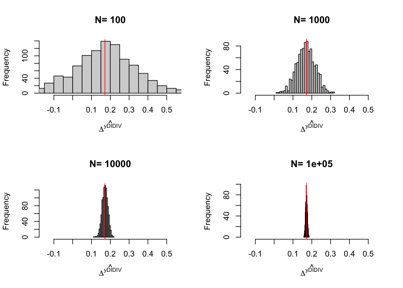
(#fig:monte.carlo.hist.iv.did.panel)Distribution of the DID-IV estimator over replications of panels of different sizes

Let us now look at repeated cross sections data

monte.carlo.iv.did.cross <- function(s,N,Nstates,param){
  set.seed(s)
  N.tot <- 2*N
  muS <- rnorm(Nstates,0,sqrt(param["sigma2mu"]/3))
  muS <- rep(muS,each=N/Nstates)
  muS <- c(muS,muS)
  # I draw an individual fixed effect with the remaining variance
  muU <- rnorm(N.tot,0,sqrt(param["sigma2mu"]*2/3))
  mu <- param["barmu"] + muS + muU 
  UB <- rnorm(N.tot,0,sqrt(param["sigma2U"]))
  yB <- mu + UB 
  YB <- exp(yB)
  epsilon <- rnorm(N.tot,0,sqrt(param["sigma2epsilon"]))
  eta<- rnorm(N.tot,0,sqrt(param["sigma2eta"]))
  U0 <- param["rho"]*UB + epsilon
  y0 <- mu +  U0 + param["delta"]
  alpha <- param["baralpha"]+  param["theta"]*mu + eta
  y1 <- y0+alpha
  Y0 <- exp(y0)
  Y1 <- exp(y1)
  # Z=1 if states have lower muS than 0
  Z <- ifelse(muS<=0,1,0)
  Ds <- ifelse(YB<=param["barY"] & Z==1,1,0)
  y <- y1*Ds+y0*(1-Ds)
  Y <- Y1*Ds+Y0*(1-Ds)
  # first cross section: 1-N
  first <- seq(1,N)
  # second cross section: 1001-2000
  second <- seq(N+1,N.tot)
  # repeated cross section DID-IV
  delta.y.iv.did.cross <- (mean(y[second][Z[second]==1])-mean(y[second][Z[second]==0])-(mean(yB[first][Z[first]==1])-mean(yB[first][Z[first]==0])))/mean(Ds[second][Z[second]==1])
  return(delta.y.iv.did.cross)
}

simuls.iv.did.cross.N <- function(N,Nstates,Nsim,param){
  simuls.iv.did.cross <- matrix(unlist(lapply(1:Nsim,monte.carlo.iv.did.cross,N=N,Nstates=Nstates,param=param)),nrow=Nsim,ncol=1,byrow=TRUE)
  colnames(simuls.iv.did.cross) <- c('DID-IV')
  return(simuls.iv.did.cross)
}

sf.simuls.iv.did.cross.N <- function(N,Nstates,Nsim,param){
  sfInit(parallel=TRUE,cpus=8)
  sim <- matrix(unlist(sfLapply(1:Nsim,monte.carlo.iv.did.cross,N=N,Nstates=Nstates,param=param)),nrow=Nsim,ncol=1,byrow=TRUE)
  sfStop()
  colnames(sim) <- c('DID-IV')
  return(sim)
}

Nsim <- 1000
#Nsim <- 10
N.sample <- c(100,1000,10000,100000)
#N.sample <- c(100,1000,10000)
#N.sample <- c(100,1000)
#N.sample <- c(100)

simuls.iv.did.cross <- lapply(N.sample,sf.simuls.iv.did.cross.N,Nstates=Nstates,Nsim=Nsim,param=param)
names(simuls.iv.did.cross) <- N.sample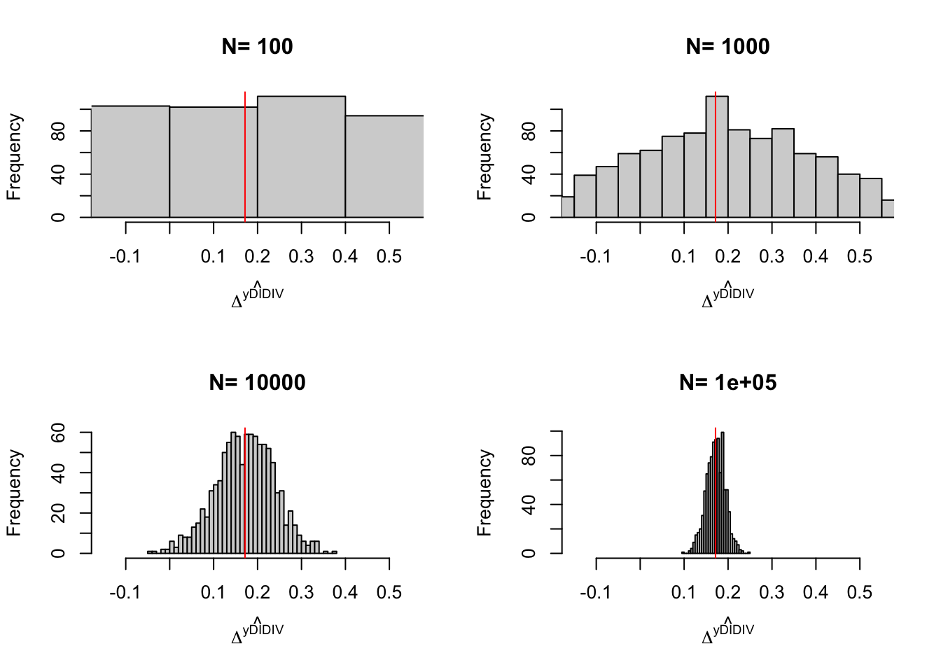

Let us now plot the result:

Distribution of the DID-IV estimator over replications of repeated cross sections of different sizes

(#fig:monte.carlo.hist.iv.did.cross.sections)Distribution of the DID-IV estimator over replications of repeated cross sections of different sizes

4.3.4.1.3 Estimation of sampling noise

What we need is to derive an estimator for the asymptotic variance of the DID-IV estimator in repeated cross sections and in panel data.

4.3.4.1.3.1 Estimating sampling noise with DID-IV in repeated cross sections

Theorem 4.30 (Asymptotic Distribution of DID-IV in Repeated Cross Sections) Under Assumptions 4.12, 4.13, 4.29, 4.17 and ??, we have:

\[\begin{align*} \sqrt{N}(\hat\Delta^Y_{DIDIV}-\Delta^Y_TT) & \stackrel{d}{\rightarrow} \mathcal{N}\left(0,\right). \end{align*}\]

Proof. To do.

4.3.4.1.3.2 Estimating sampling noise with DID-IV in panel data

Theorem 4.31 (Asymptotic Distribution of DID-IV in Panel Data) Under Assumptions 4.12, 4.13, 4.29, 4.15 and 4.16, we have:

\[\begin{align*} \sqrt{N}(\hat\Delta^Y_{DIDIV}-\Delta^Y_TT) & \stackrel{d}{\rightarrow} \mathcal{N}\left(0,\right). \end{align*}\]

Proof. To do.

Example 4.60 Let’s see how estimators of sampling noise perform in practice.

In panel data, true 99% sampling noise (from the simulations) is 0.25. 99% sampling noise estimated using default FE standard errors is 0.22`. 99% sampling noise estimated using heteroskedasticity robust FE standard errors is 0.22.

In repeated cross sections, true 99% sampling noise (from the simulations) is 1.16. 99% sampling noise estimated using default OLS standard errors is 0.24. 99% sampling noise estimated using heteroskedasticity robust OLS standard errors is 0.25.

4.3.4.2 DID-IV with a weak first stage

With a weak first stage, DID-IV has positive probability of receiving the treatment in the Before period and in the group with $Z_i=0$. The main requirement of the weak first stage DID-IV is that the probability of receiving the treatment increases more over time in the group with $Z_i=1$ compared to what happens in the group with $Z_i=0$. We are going to codify this assumption next and see which effects can be identified under which supplementary assumptions, then talk about estimation and estimation of sampling noise.

4.3.4.2.1 Identification

We are going to examine several sets of assumptions under which we can try to recover some average treatment effect of the treatment in a DID-IV design with a weak first stage. As you’ll see, there is not much hope unfortunately.

4.3.4.2.1.1 Identification under weak first stage DID-IV

The main assumption on a weak first stage DID-IV is as follows:

Hypothesis 4.31 (Weak First Stage) The treatment is available in both periods $B$ and $A$, but its takeover increases disproportionately among those with $Z_i=1$:

\[\begin{align*} \Pr(D_{i,A}=1|Z_i=1)& -\Pr(D_{i,B}=1|Z_i=1)\\ & >\Pr(D_{i,A}=1|Z_i=0)-\Pr(D_{i,B}=1|Z_i=0). \end{align*}\]

Remark. A great example of Assumption 4.31 is Esther Duflo’s paper in education expansion in Indonesia. In this paper, the states that invest in education are the ones for which education levels were the lowest initially. And the states with lower investments in education ($Z_i=0$) nevertheless saw some progress in education levels over time. But, the states with higher investments ($Z_i=1$) saw stronger improvements and caught up. Also, all states had some education in the baseline period. This is characteristic of a weak first stage DID-IV design.

Example 4.61 Let us now see how we can model this in our example.

We are going to introduce an eligibility rule that changes over time as a function of state and district fixed effects:

\[\begin{align*} \mu_i & = \mu^S_i + \mu^d_i + \mu^U_i + \bar{\mu} \\ \mu^S_i & \sim\mathcal{N}(0,\frac{1}{3}\sigma_{\mu}^2)\\ \mu^d_i & \sim\mathcal{N}(0,\frac{1}{3}\sigma_{\mu}^2)\\ \mu^U_i & \sim\mathcal{N}(0,\frac{1}{3}\sigma_{\mu}^2)\\ E_{i,B} & = \begin{cases} 1 & \text{ if } \mu^d_i\leq -0.5 \land Z_i=1 \\ 1 & \text{ if } \mu^d_i\leq 0.25\land Z_i=0 \end{cases}\\ E_{i,A} & = \begin{cases} 1 & \text{ if } \mu^d_i\leq 0 \land Z_i=1 \\ 1 & \text{ if } \mu^d_i\leq 0.85\land Z_i=0 \end{cases}\\ D_{i,t} & = \uns{y_{i,BB}\leq\bar{y} \land E_{i,t}=1}. \end{align*}\]

The rest of the model is as follows, with a third period $BB$ that is Before Before:

\[\begin{align*} y^0_{i,A} & =\mu_i+\delta+U_{i,A}^0 \\ y_{i,A}^1 & =\mu_i(1+\theta)+\bar{\alpha}+\delta+U_{i,A}^0+\eta_i \\ y_{i,BB} & =\mu_i+U_{i,BB} \\ U_{i,B}^0 & =\rho U_{i,BB}+\epsilon_{i,B} \\ U_{i,A}^0 & =\rho U_{i,B}+\epsilon_{i,A} \\ U_{i,BB} & \sim\mathcal{N}(0,\sigma^2_{U})\\ \epsilon_{i,t} & \sim\mathcal{N}(0,\sigma^2_{\epsilon})\\ \eta_i & \sim\mathcal{N}(0,\sigma^2_{\eta}) \end{align*}\]

Here is the simulation:

Let us now see how the model generates a time varying proportion of participants:

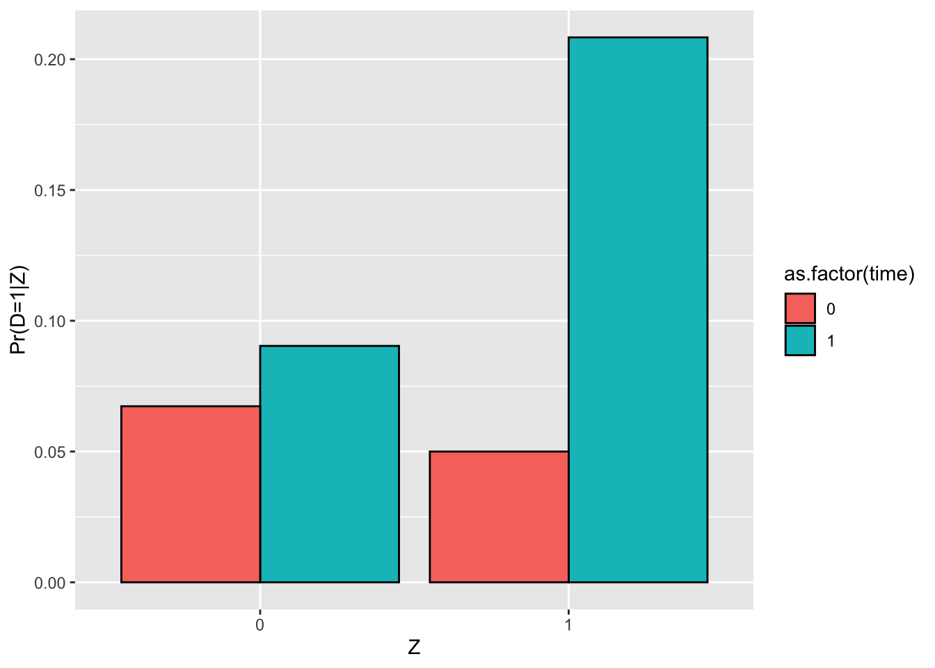
Figure 4.49: Illustration of the DID-IV assumptions: Weak First Stage

We thus see that the change over time in treatment uptake is equal to 0.16 when $Z_i=1$ and to 0.02 when $Z_i=0$.

4.3.4.2.1.2 Identification with independent treatment effects

Under constant treatment effects, the classical Wald DID estimator still identifies the effect of the treatment on the treated:

Hypothesis 4.32 (Independent Treatment Effects) The average effect of the treatment on the treated is independent of $Z_i$:

\[\begin{align*} \esp{Y_{i,t}^1-Y_{i,t}^0|D_i=1,Z_i=1} & = \esp{Y_{i,t}^1-Y_{i,t}^0|D_i=1,Z_i=0}. \end{align*}\]

Under Assumption 4.32, we can show that the Wald DID estimator recovers the average effect of the treatment on the treated:

Theorem 4.32 (Indentification of TT with DID-IV, a Weak First Stage and Independent Treatment Effects) Under Assumptions 4.12, 4.13, 4.29, 4.31 and 4.32, TT is identified by the Wald-DID estimator:

\[\begin{align*} \Delta^Y_{WaldDID} & = \Delta^{Y_A}_{TT}. \end{align*}\]

Proof. We have, for $t\in\left\{ A,B \right\}$ and $d\in\left\{ 0,1 \right\}$:

\[\begin{align*} \esp{Y_{i,t}|Z_i=d} & = \esp{Y^0_{i,t}|Z_i=d} + \esp{Y^1_{i,t}-Y^0_{i,t}|D_{i,t}=1,Z_i=d}\Pr(D_{i,t}=1|Z_i=d) \end{align*}\]

Under Assumption 4.32, $\esp{Y^1_{i,t}-Y^0_{i,t}|D_{i,t}=1,Z_i=d}=\Delta^Y_{TT}$. As a consequence, the numerator of the Wald-DID estimator writes as follows:

\[\begin{align*} \esp{Y_{i,A}|Z_i=1} & -\esp{Y_{i,A}|Z_i=0}-(\esp{Y_{i,B}|Z_i=1}-\esp{Y_{i,B}|Z_i=0}) \\ & = \esp{Y^0_{i,A}-Y^0_{i,B}|Z_i=1}+ \Delta^Y_{TT}\left(\Pr(D_{i,A}=1|Z_i=1)-\Pr(D_{i,B}=1|Z_i=1)\right)\\ & \phantom{=} -\esp{Y^0_{i,A}-Y^0_{i,B}|Z_i=0}-\Delta^Y_{TT}\left(\Pr(D_{i,A}=1|Z_i=0)-\Pr(D_{i,B}=1|Z_i=0)\right). \end{align*}\]

Using the Assumption 4.29 and dividing by the denominator of the Wald-DID estimator (which is non null under Assumption 4.31) yields the result.

4.3.4.2.1.3 Identification under constant treatment effects over time

The problem with DID-IV stems when treatment effects are not independent from $Z_i$ conditional on $D_i=1$. We can get an inkling of the problem at hand by deriving the Wald estimator without Assumption 4.32, but under Assumptions 4.12, 4.13, 4.29 and 4.31. Let’s get some notation first. We denote $\Delta^D_{DID}=\Pr(D_{i,A}=1|Z_i=1)-\Pr(D_{i,B}=1|Z_i=1)-(\Pr(D_{i,A}=1|Z_i=0)-\Pr(D_{i,B}=1|Z_i=0))$, the denominator of the Wald estimator. We also denote $p^{AB}_{11}=\Pr(D_{i,A}=1|Z_i=1)-\Pr(D_{i,B}=1|Z_i=1)$ and $p^{AB}_{10}=\Pr(D_{i,A}=1|Z_i=0)-\Pr(D_{i,B}=1|Z_i=0)$. We finally denote $\Delta^{Y_A}_{TT_1}=\esp{Y_{i,t}^1-Y_{i,t}^0|D_i=1,Z_i=1}$ and $\Delta^{Y_A}_{TT_0}=\esp{Y_{i,t}^1-Y_{i,t}^0|D_i=1,Z_i=0}$. We can now prove the following corollary to Theorem 4.32:

Corollary 4.4 (DID-Wald Estimator Without Independent Treatment Effects) Under Assumptions 4.12, 4.13, 4.29 and 4.31, the DID-Wald estimator is a weighted average of treatment effects with possibly negative weights:

\[\begin{align*} \Delta^Y_{WaldDID} & = \Delta^{Y_A}_{TT_1}\frac{p^{AB}_{11}}{\Delta^D_{DID}}-\Delta^{Y_A}_{TT_0}\frac{p^{AB}_{10}}{\Delta^D_{DID}}. \end{align*}\]

Proof. Using the proof of Theorem 4.32 proves the result.

Corollary 4.4 shows that, when the proportion of treated in the group with $Z_i=0$ increases over time, the impact of the treatment on those with $Z_i=0$ enters negatively in the Wald-DID estimator. It is thus possible that positive treatment effects for every unit in the population generates a negative Wald-DID estimator.

We can even get a deeper understanding of what’s going on with the DID-IV estimator if we follow the classic treatment of this issue by de Chaisemartin and d’Haultfoeuille (2015). Let us first define four types of individuals:

always takers: the individuals which have $D_{i,A}=D_{i,B}=1$, which we denote $T_i=at$,
never takers: the individuals which have $D_{i,A}=D_{i,B}=0$, which we denote $T_i=nt$,
switchers: the individuals which have $D_{i,A}=1$ and $D_{i,B}=0$, which we denote $T_i=s$,
anti-switchers: the individuals which have $D_{i,A}=0$ and $D_{i,B}=1$, which we denote $T_i=as$.

For now, we are going to assume away anti-switchers for simplicity.
Assumption 4.31 amounts to assuming that $\Pr(T_i=s|Z_i=1) > \Pr(T_i=s|Z_i=0)$. We can now prove the following theorem:

Theorem 4.33 (Numerator of the DID-Wald Estimator Without Independent Treatment Effects and Without Anti-Switchers) Under Assumptions 4.12, 4.13, 4.29 and 4.31, and in the absence of anti-switchers ($\Pr(T_i=as)=0$), the numerator of the DID-Wald estimator can be written as follows:

\[\begin{align*} \Delta^Y_{WaldDID}\Delta^D_{DID} & = \esp{Y^1_{i,A}-Y^1_{i,B}|T_i=at,Z_i=1}\Pr(T_i=at|Z_i=1)\\ & \phantom{=} +\esp{Y^0_{i,A}-Y^0_{i,B}|T_i=nt,Z_i=1}\Pr(T_i=nt|Z_i=1)\\ & \phantom{=} +\esp{Y^1_{i,A}-Y^0_{i,B}|T_i=s,Z_i=1}\Pr(T_i=s|Z_i=1)\\ & \phantom{=} -(\esp{Y^1_{i,A}-Y^1_{i,B}|T_i=at,Z_i=0}\Pr(T_i=at|Z_i=0))\\ & \phantom{=} -(\esp{Y^0_{i,A}-Y^0_{i,B}|T_i=nt,Z_i=0}\Pr(T_i=nt|Z_i=0))\\ & \phantom{=} -(\esp{Y^1_{i,A}-Y^0_{i,B}|T_i=s,Z_i=0}\Pr(T_i=s|Z_i=0)). \end{align*}\]

Proof. The result follows from the formula for the DID-Wald estimator and the fact that $T_i$ is a partition of the population.

So, the numerator of the Wald-DID estimator is a combination of the changes in outcomes over time of each type in the group with $Z_i=1$ minus the changes the outcomes of each type in the group with $Z_i=0$. The units with the same type are not the same in each group defined by $Z_i$ so that their proportions differ and their changes in outcome differ as well. One useful simplification can still happen using Assumption 4.29. Let $\Delta^{Y_A}_{\text{type},z}=\esp{Y_{i,t}^1-Y_{i,t}^0|T_i=\text{type},Z_i=z}$, for $\text{type}\in\left\{at,nt,s\right\}$ and $z\in\left\{0,1\right\}$. Let also $p_{\text{type},z}=\Pr(T_i=\text{type}|Z_i=z)$. The following corollary proves that:

Corollary 4.5 (DID-Wald Estimator Without Independent Treatment Effects) Under Assumptions 4.12, 4.13, 4.29 and 4.31, the DID-Wald estimator can be decomposed as follows:

\[\begin{align*} \Delta^Y_{WaldDID}\Delta^D_{DID} & = \Delta^{Y_A}_{s,1}p_{s,1}-\Delta^{Y_A}_{s,0}p_{s,0}+(\Delta^{Y_A}_{at,1}-\Delta^{Y_B}_{at,1})p_{at,1}-(\Delta^{Y_A}_{at,0}-\Delta^{Y_B}_{at,0})p_{at,0}. \end{align*}\]

Proof. Using Theorem 4.33, we can now add and subtract $\esp{Y^0_{i,A}-Y^0_{i,B}|T_i=at,Z_i=1}\Pr(T_i=at|Z_i=1)$, $\esp{Y^0_{i,A}-Y^0_{i,B}|T_i=at,Z_i=0}\Pr(T_i=at|Z_i=0)$, $\esp{Y^0_{i,A}|T_i=s,Z_i=1}\Pr(T_i=s|Z_i=1)$ and $\esp{Y^0_{i,A}|T_i=s,Z_i=0}\Pr(T_i=s|Z_i=0)$ to the right hand side of the expression, and use the fact that $T_i$ is a partition and then invoke Assumption 4.29 to obtain the result.

Corollary 4.5 shows that the Wald-DID estimator is a weighted average of the effect of the treatment on the switchers in the group with $Z_i=1$, minus the effect of the treatment on the switchers in the group with $Z_i=0$, and the change in the treatment effect over time among always takers in the group with $Z_i=1$ minus the change in treatment effect over time among always takers in the group with $Z_i=0$. So, one way to get rid of the issue is to assume constant treatment effects over time for both groups of always takers. Let’s make this assumption and see where it takes us:

Hypothesis 4.33 (Constant Treatment Effects Over Time) We assume that average effect of the treatment on the always takers is independent of time, conditional on $Z_i$: $\forall z \in \left\{0,1\right\}$:

\[\begin{align*} \Delta^{Y_A}_{at,z}& = \Delta^{Y_B}_{at,z} \end{align*}\]

We can now prove the following Theorem:

Theorem 4.34 (DID-Wald Estimator With Constant Treatment Effects Over Time) Under Assumptions 4.12, 4.13, 4.29, 4.31 and 4.33, the DID-Wald estimator can be decomposed as follows:

\[\begin{align*} \Delta^Y_{WaldDID} & = \begin{cases} \Delta^{Y_A}_{s,1} \text{ if }p_{s,0}=0\\ \alpha\Delta^{Y_A}_{s,1}-(1-\alpha)\Delta^{Y_A}_{s,0}\text{, }0<\alpha<1 \text{ if } p_{s,0}<0\\ \alpha\Delta^{Y_A}_{s,1}-(1-\alpha)\Delta^{Y_A}_{s,0}\text{, }\alpha>1 \text{ if } p_{s,0}>0. \end{cases} \end{align*}\]

Proof. Using Corollary 4.5 and the fact that $\Delta^D_{DID}=p_{s,1}-p_{s,0}$ proves the result.

Note that Theorem 4.34 still does not get rid of the issue of negative weights in the case when the proportion of treated units increases in the control group.

4.3.4.2.1.4 Identification under parallel trends by type

de Chaisemartin and d’Haultfoeuille (2015) propose an alternative to Assumption 4.33. This approach requires that there are no shifters in the group with $Z_i=0$, and thus that the proportion of treated units does not change over time in this group. This is thus very close to a DID-IV design with Strong First Stage. Finally, their approach requires an alternative parallel trends assumption over groups. Let is state all of these assumptions:

Hypothesis 4.34 (Strong Weak First Stage) We assume that the proportion of treated stays constant in the group with $Z_i=0$: $p_{s,0}=0$.

Hypothesis 4.35 (Conditional Parallel Trends) We assume that the trends in potential outcomes among groups defined by $D_{i,B}$ does not depend on $Z_i$:

\[\begin{align*} \esp{Y^d_{i,A}-Y^d_{i,B}|D_{i,B}=d,Z_i=1} & = \esp{Y^d_{i,A}-Y^d_{i,B}|D_{i,B}=d,Z_i=0}. \end{align*}\]

Remark. Assumption 4.35 is very strong. It assumes away part of the time-varying selection bias that the instrumental variable procedure is trying to undo.

de Chaisemartin and d’Haultfoeuille (2015) prove that a $Wald_{TC}$, a time-corrected Wald estimator, is able to recover the average effect of the treatment on the shifters under these assumptions:

Theorem 4.35 (Time-corrected Wald Estimator With Conditional Parallel Trends) Under Assumptions 4.12, 4.13, 4.34 and 4.35, the time-corrected Wald estimator identifies the average effect of the treatment on the shifters:

\[\begin{align*} \Delta^Y_{Wald_{TC}} & = \Delta^{Y_A}_{s,1}, \end{align*}\]

with:

\[\begin{align*} \Delta^Y_{Wald_{TC}} & = \frac{\esp{Y_{i,A}|Z_i=1}-\esp{Y_{i,B}+D_{i,B}\delta_1+(1-D_{i,B})\delta_0|Z_i=1}}{\Pr(D_{i,A}=1|Z_i=1)-\Pr(D_{i,B}=1|Z_i=1)}\\ \delta_1 & = \esp{Y_{i,A}-Y_{i,B}|D_{i,B}=1,Z_i=0}\\ \delta_0 & = \esp{Y_{i,A}-Y_{i,B}|D_{i,B}=0,Z_i=0}. \end{align*}\]

Proof. Note that:

\[\begin{align*} \esp{Y_{i,A}|Z_i=1} & = \esp{Y_{i,A}|D_{i,B}=1,Z_i=1}\Pr(D_{i,B}=1|Z_i=1)\\ & \phantom{=}+\esp{Y_{i,A}|D_{i,B}=0,Z_i=1}\Pr(D_{i,B}=0|Z_i=1)\\ \esp{Y_{i,B}|Z_i=1} & = \esp{Y_{i,B}|D_{i,B}=1,Z_i=1}\Pr(D_{i,B}=1|Z_i=1)\\ & \phantom{=}+\esp{Y_{i,B}|D_{i,B}=0,Z_i=1}\Pr(D_{i,B}=0|Z_i=1)\\ \esp{D_{i,B}\delta_1|Z_i=1} & = \esp{Y_{i,A}-Y_{i,B}|D_{i,B}=1,Z_i=0}\Pr(D_{i,B}=1|Z_i=1)\\ \esp{(1-D_{i,B})\delta_0|Z_i=1} & = \esp{Y_{i,A}-Y_{i,B}|D_{i,B}=0,Z_i=0}\Pr(D_{i,B}=0|Z_i=1). \end{align*}\]

With $D_{i,B}=1$, we know that $Y_{i,A}=Y^1_{i,A}$ and $Y_{i,B}=Y^1_{i,B}$. As a consequence, using Assumption 4.35, we have:

\[\begin{align*} \Delta^Y_{Wald_{TC}} & = \frac{(\esp{Y_{i,A}-Y_{i,B}|D_{i,B}=0,Z_i=1}-\esp{Y_{i,A}-Y_{i,B}|D_{i,B}=0,Z_i=0})\Pr(D_{i,B}=0|Z_i=1)}{\Pr(D_{i,A}=1|Z_i=1)-\Pr(D_{i,B}=1|Z_i=1)}. \end{align*}\]

Using the fact that, conditional on $Z_i=1$, the population with $D_{i,B}=0$ can be split totally into $T_i=s$ and $T_i=nt$, we can write the following equality (after adding and subtracting $\esp{Y^0_{i,A}|T_i=s,Z_i=1}$):

\[\begin{align*} \esp{Y_{i,A}-Y_{i,B}|D_{i,B}=0,Z_i=1} & = \Delta^{Y_A}_{s,1}\Pr(T_i=s|D_{i,B}=0,Z_i=1)+\esp{Y^0_{i,A}-Y^0_{i,B}|D_{i,B}=0,Z_i=1}. \end{align*}\]

Using Assumption 4.34, with $D_{i,B}=0$ and $Z_i=0$, we know that $Y_{i,A}=Y^0_{i,A}$ and $Y_{i,B}=Y^0_{i,B}$. Using Assumption 4.35 again, we have:

\[\begin{align*} \Delta^Y_{Wald_{TC}} & = \frac{\Delta^{Y_A}_{s,1}\Pr(T_i=s|D_{i,B}=0,Z_i=1)\Pr(D_{i,B}=0|Z_i=1)}{\Pr(D_{i,A}=1|Z_i=1)-\Pr(D_{i,B}=1|Z_i=1)}. \end{align*}\]

Note that $T_i=s\Rightarrow D_{i,B}=0|Z_i=1$, so that $\Pr(T_i=s|D_{i,B}=0,Z_i=1)\Pr(D_{i,B}=0|Z_i=1)=\Pr(T_i=s|Z_i=1)$. Under Assumption 4.34, $\Pr(T_i=s|Z_i=1)=\Pr(D_{i,A}=1|Z_i=1)-\Pr(D_{i,B}=1|Z_i=1)$, which proves the result.

Remark. The problem with Theorem 4.34 is that it relies on Assumption 4.34: there are no changes in the proportion of units receiving the treatment in the group with $Z_i=0$. This assumption might very often be untrue. Fortunately, de Chaisemartin and d’Haultfoeuille (2015) show that you can relax that assumption and still bound the treatment effect if your outcome is bounded. We will present this estimator in Section ??.

4.3.4.2.2 Estimation

We are going to look at how to estimate the Time-Corrected Wald estimator of de Chaisemartin and d’Haultfoeuille (2015). The formula for the estimator is pretty straightforward:

\[\begin{align*} \hat\Delta^Y_{Wald_{TC}} & = \frac{\frac{\sum_{i=1}^NY_{i,A}Z_i}{\sum_{i=1}^NZ_i}-\frac{\sum_{i=1}^NY_{i,B}Z_i}{\sum_{i=1}^NZ_i}-\hat\delta_1\frac{\sum_{i=1}^ND_{i,B}(1-Z_i)}{\sum_{i=1}^N(1-Z_i)}-\hat\delta_0\frac{\sum_{i=1}^N(1-D_{i,B})(1-Z_i)}{\sum_{i=1}^N(1-Z_i)}}{\frac{\sum_{i=1}^ND_{i,A}Z_i}{\sum_{i=1}^NZ_i}-\frac{\sum_{i=1}^ND_{i,B}Z_i}{\sum_{i=1}^NZ_i}}\\ \hat\delta_1 & = \frac{\sum_{i=1}^NY_{i,A}D_{i,B}(1-Z_i)}{\sum_{i=1}^ND_{i,B}(1-Z_i)}-\frac{\sum_{i=1}^NY_{i,B}D_{i,B}(1-Z_i)}{\sum_{i=1}^ND_{i,B}(1-Z_i)}\\ \hat\delta_0 & = \frac{\sum_{i=1}^NY_{i,A}(1-D_{i,B})(1-Z_i)}{\sum_{i=1}^N(1-D_{i,B})(1-Z_i)}-\frac{\sum_{i=1}^NY_{i,B}(1-D_{i,B})(1-Z_i)}{\sum_{i=1}^N(1-D_{i,B})(1-Z_i)}. \end{align*}\]

Example 4.62 Let us now look at how the Wald-TC estimator and the more traditional Wald-DID estimator work in our example. Let’s compute them both:

# Wald DID estimator
# changes in mean outcomes over time
DeltaYZ1 <- mean(y[Z==1])-mean(yB[Z==1])
DeltaYZ0 <- mean(y[Z==0])-mean(yB[Z==0])
DeltaDZ1 <- mean(DsA[Z==1])-mean(DsB[Z==1])
DeltaDZ0 <- mean(DsA[Z==0])-mean(DsB[Z==0])
WaldDID <- (DeltaYZ1-DeltaYZ0)/(DeltaDZ1-DeltaDZ0)

# Wald TC estimator
DeltaYDZ10 <- mean(y[DsB==1&Z==0])-mean(yB[DsB==1&Z==0])
DeltaYDZ00 <- mean(y[DsB==0&Z==0])-mean(yB[DsB==0&Z==0])
MeanDBZ0 <- mean(DsB[Z==0])
WaldTC <- (DeltaYZ1-MeanDBZ0*DeltaYDZ10-(1-MeanDBZ0)*DeltaYDZ00)/(DeltaDZ1)

# true effect on switchers in the sample
DeltaYAs1Sample <- mean(y1A[DsB==0&DsA==1&Z==1])-mean(y0A[DsB==0&DsA==1&Z==1])
DeltaYAs0Sample <- mean(y1A[DsB==0&DsA==1&Z==0])-mean(y0A[DsB==0&DsA==1&Z==0])
DeltaYBs1Sample <- mean(y1B[DsB==0&DsA==1&Z==1])-mean(y0B[DsB==0&DsA==1&Z==1])
DeltaYBs0Sample <- mean(y1B[DsB==0&DsA==1&Z==0])-mean(y0B[DsB==0&DsA==1&Z==0])
DeltaYAat1Sample <- mean(y1A[DsB==1&DsA==1&Z==1])-mean(y0A[DsB==1&DsA==1&Z==1])
DeltaYAat0Sample <- mean(y1A[DsB==1&DsA==1&Z==0])-mean(y0A[DsB==1&DsA==1&Z==0])
DeltaYBat1Sample <- mean(y1B[DsB==1&DsA==1&Z==1])-mean(y0B[DsB==1&DsA==1&Z==1])
DeltaYBat0Sample <- mean(y1B[DsB==1&DsA==1&Z==0])-mean(y0B[DsB==1&DsA==1&Z==0])

# checking PTA
DeltaY0BAZ1 <- mean(y0A[Z==1])-mean(y0B[Z==1])
DeltaY0BAZ0 <- mean(y0A[Z==0])-mean(y0B[Z==0])
DeltaY1atBAZ1 <- mean(y1A[DsB==1&DsA==1&Z==1])-mean(y1B[DsB==1&DsA==1&Z==1])
DeltaY1atBAZ0 <- mean(y1A[DsB==1&DsA==1&Z==0])-mean(y1B[DsB==1&DsA==1&Z==0])

# alpha
alpha.shifters <- DeltaDZ1/(DeltaDZ1-DeltaDZ0)

# weighted average of shifters impacts
DeltaYAsSample <- DeltaYAs1Sample*alpha.shifters+(1-alpha.shifters)*DeltaYAs0Sample

The Wald-DID estimator in our example is equal to 0.47 while the true average effect of the treatment on the shifters in the group with $Z_i=1$ is equal to 0.2 in the sample. The Time-corrected Wald estimator is equal to 0.4. It is hard to say why these estimators are too big in our example. The Wald-DID estimator should not be too biased since Assumption 4.33 holds in our dataset, and the bias stemming from the failure of Assumption 4.34 is not too severe. Indeed, using Theorem 4.34, we know that Wald-DID estimator should converge to the weighted average of the effect on shifters, which is equal to 0.22 in the sample. As always with Wald estimators, I suspect that the denominator is slightly too small, and that the proportion of switchers is underestimated.

4.3.5 Difference In Differences with Continuous Treatment Variables and Staggered Adoption

Another case that might appear is when the treatment variable is continuous (for example a share between zero and one) and its changes are staggered over time. In that case, a recent contribution by Clement de Chaisemartin and Xavier d’Haultfoeuille clarifies what can be estimated and under which assumptions. In this section, we are going to look at the identification abd estimation of these effects as proposed by de Chaisemartin and d’Haultfoeuille.

4.3.5.1 Identification

Maybe the toughest part of addressing the issue of continuous treatments with staggered adoption is the definition of the treatment parameters. Indeed, we now have a potentially infinite set of treatment levels, compounded by a large set of treatment dates. Much of the contribution of Clement and Xavier is to get the definition of the parameter of interest right. They actually propose two sets of definitions: a normalized and a non-normalized average treatment effect. Let us start with the normalized one.

Before defining what the treatment parameters are, we need to define our setup, which is going to be richer than the ones we have used so far. The whole setup in Xavier and Clement’s approach is predicated on having access to a panel of $G$ groups observed over $T$ periods of time. The groups can be built by aggregating a set of individual level panel data or repeated cross-section observations at some more aggregate level (like municipality or state). Each individual unit can also form its own group, as long as it observed in a panel. $D_{g,t}$ denotes the continuous level of treatment of group $g$ at period $t$. The treatment is assumed to be nonnegative for simplicity. Let $\mathbf{D}_g=\left(D_{g,1},\dots,D_{g,T}\right)$ be the set of treatments that group $g$ experiences over time, and $\mathbf{D}=\left(\mathbf{D}_{1},\dots,\mathbf{D}_{G}\right)$ the vector of all treatment paths for each group over time. $\mathcal{D}$ is the support of $\mathbf{D}_g$. Potential outcomes are going to depend on the whole vector of past and future treatments: $Y_{g,t}(d_1,\dots,d_T)$ is the potential outcome observed for group $g$ at time $t$ if $\mathbf{D}_g=(d_1,\dots,d_T)$. The observed outcome for group $g$ at time $t$ is $Y_{g,t}=Y_{g,t}(\mathbf{D}_g)$.

Xavier and Clement require several assmptions on the design. To define the first one, we need to define $F_g=\min\left\{ t:t\geq 2, D_{g,t}\neq D_{g,t-1}\right\}$, the the first date at which treatment changes. The convention is that $F_{g}=T+1$ for the group for which treatment status never changes.

Hypothesis 4.36 (Variation in treatment exposure) We assume that the design is such that: $\exists (g,g')$ such that $D_{g,1}=D_{g',1}$ and $F_g\neq F_{g'}$.

Assumption 4.36 imposes that there exists groups with similar levels of first period treatment intensity, but which get treated at different periods. To this assumption, the authors add two main ones:

Hypothesis 4.37 (No Anticipation with Continuous and Staggered Treatments) We assume that $\forall g$, $\forall (d_1,\dots,d_T)\in\mathcal{D}$, $Y_{g,t}(d_1,\dots,d_T)=Y_{g,t}(d_1,\dots,d_t)$.

For the last assumption, let $\mathcal{D}_1^r=\left\{d:\exists(g,g')\in\left\{1,\dots,G\right\}^2:D_{g,1}=D_{g',1}, F_g\neq F_{g'}\right\}$ be the set of first period treatment levels for which there are at least two groups having that value and different fates of treatment intake. Let also $\mathbf{D}_{g,1,k}$ be the $1\times k$ vector repeating $D_{g,1}$. Finally, let $Y_{g,t}(\mathbf{D}_{g,1,t})$ be the potential outcome of group $g$ at time $t$ had it kept its initial treatment level at all periods, or ``status quo’’ outcome.

Hypothesis 4.38 (Parallel Trends with Continuous and Staggered Treatments) We assume that $\forall g,g'$, if $D_{g,1}=D_{g',1}\in\mathcal{D}_1^r$, then, $\forall t\geq 2$,

\[\begin{align*} \esp{Y_{g,t}(\mathbf{D}_{g,1,t})-Y_{g,t-1}(\mathbf{D}_{g',1,t-1})|\mathbf{D}} & = \esp{Y_{g',t}(\mathbf{D}_{g',1,t})-Y_{g,t-1}(\mathbf{D}_{g',1,t-1})|\mathbf{D}}. \end{align*}\]

Following Assumption 4.38, the status quo outcomes of groups with the same period 1 treatment level would have followed parallel trends.

4.3.5.1.1 Identifying non normalized treatment effects

We are now equipped to define some target treatment parameters. Let us define $T_g=\max_{g':D_{g',1}=D_{g,1}}F_{g'}-1$, the last period in the dataset where a group with the same initial treatment intensity as $g$ remains at the status quo treatment level. For any $g$ such that $F_g\leq T_g$, and for any $l\in\left\{1,\dots,T_g-F_g+1\right\}$, the average treatment effect of the treatment sequence on group $g$ after $l$ periods under treatment is equal to:

\[\begin{align*} \delta_{g,l} & = \esp{Y_{g,F_g-1+l}-Y_{g,F_g-1+l}(\mathbf{D}_{g,1,F_g-1+l})|\mathbf{D}}. \end{align*}\]

We are going to identify this target parameter $\delta_{g,l}$ using a generalized DID estimator based on the $N^g_{F_g-1+l}$ groups that stayed in the status quo treatment until $F_g-1+l$ (with $N^g_t=\#\left\{g':D_{g',1}=D_{g,1},F_{g',t}>t\right\}$, and $\#\left\{A\right\}$ the cardinal of $A$):

\[\begin{align*} DID_{g,l} & = Y_{g,F_g-1+l}-Y_{g,F_g-1}-\frac{1}{N^g_{F_g-1+l}}\sum_{g':D_{g',1}=D_{g,1},F_{g'}>F_g-1+l}\left(Y_{g',F_g'-1+l}-Y_{g',F_g-1}\right). \end{align*}\]

We are now able to state the first identification result:

Theorem 4.36 (Identification in DID with Continuous and Staggered Treatments (one group)) Under Assumptions 4.36, 4.37 and 4.38, we have, $\forall (g,l)$ such that $1\leq l \leq T_g-F_g+1$:

\[\begin{align*} \delta_{g,l} & = \esp{DID_{g,l}|\mathbf{D}}. \end{align*}\]

Proof. See de Chaisemartin and d’Haultfoeuille.

What remains to be done is to aggregate over all possible groups. In order to do that, we need to distinguish between groups for which treatment increases and those for which treatment decreases, and we need to assume away groups for which treatment increases at some date and then decreases later on:

Hypothesis 4.39 (No Crossing Condition) We assume that the design is such that: $\forall g\in\left\{1,\dots,G\right\}$, either $D_{g,t}\geq D_{g,1}$ $\forall t$ or $D_{g,t}\leq D_{g,1}$ $\forall t$.

We also denote $L=\max{g}(T_g-F_g+1)$ the maximum number of periods for which we can estimate the treatment effect; $N_l=\#\left\{g:F_g-1+l\leq T_g\right\}$ the number of groups for which the effect of being $l$ periods under treatment can be estimated; and $S_g=\uns{D_{g,F_g}>D_{g,1}}-\uns{D_{g,F_g}<D_{g,1}}$ taking value $1$ when treatment increases over time and $-1$ when treatment decreases over time, we can define the weighted average effect after $l$ periods under treatment as:

\[\begin{align*} \delta_{l} & = \frac{1}{N_{l}}\sum_{g:F_g-1+l\leq T_g}S_g\delta_{g,l}. \end{align*}\]

We can now prove the following theorem:

Theorem 4.37 (Identification in DID with Continuous and Staggered Treatments) Under Assumptions 4.36, 4.37, 4.38 and 4.39, we have, $\forall l$ such that $1\leq l \leq L$:

\[\begin{align*} \delta_{l} & = \frac{1}{N_{l}}\sum_{g:F_g-1+l\leq T_g}S_gDID_{g,l}. \end{align*}\]

Proof. The result follows directly from the application of Theorem 4.36.

4.3.5.1.2 Identifying normalized treatment effects

Theorems 4.36 and 4.37 identify the average actual vs status quo effect across groups. Their event study profile is going to depend on the precise distribution of treatment sequences among treated groups. One way to try to normalize that average treatment effect estimate is by combining all estimates as a proportion of the cumulative treatment intensity they have received. One way to achieve that is to define the following cumulative treatment intensity variable, for any $g$ such that $F_g\leq T_g$ and any $l\in\left\{1,\dots,T_g-F_g+1\right\}$:

\[\begin{align*} \delta^D_{g,l} & = \sum_{k=1}^{l}\left(D_{g,F_{g+k-1}}-D_{g,1}\right). \end{align*}\]

We can then define the normalized treatment effect for group $g$ after $l$ periods under the treatment as follows:

\[\begin{align*} \delta^n_{g,l} & = \frac{\delta_{g,l}}{\delta^D_{g,l}}. \end{align*}\]

This effect is identified:

Theorem 4.38 (Identification of Normalized Effects in DID with Continuous and Staggered Treatments (one group)) Under Assumptions 4.36, 4.37 and 4.38, we have, $\forall (g,l)$ such that $1\leq l \leq T_g-F_g+1$:

\[\begin{align*} \delta^n_{g,l} & = \esp{\frac{DID_{g,l}}{\delta^D_{g,l}}|\mathbf{D}}. \end{align*}\]

Proof. The result follows directly from the application of Theorem 4.36, and from the fact that $\delta^D_{g,l}$ is a constant conditional on $\mathbf{D}$.

Now, we would like to aggregate all of the effects on each group together to obtain one normalized effect after $l$ periods under treatment. We are going to weigh all groups by their share of the total change treatment intensity at date $l$: $\delta^D_l=\frac{1}{N_l}\sum_{g:F_g-1+l\leq T_g}\left|\delta^D_{g,l}\right|$. As a consequence, we use as normalized treatment effect after $l$ periods under treatment:

\[\begin{align*} \delta^n_{l} & =\frac{1}{N_l}\sum_{g:F_g-1+l\leq T_g}\frac{\left|\delta^D_{g,l}\right|}{\delta^D_{l}}\delta^n_{g,l}. \end{align*}\]

Following all the results from this section, we have the folowing theorem:

Theorem 4.39 (Identification of Normalized Effects in DID with Continuous and Staggered Treatments) Under Assumptions 4.36, 4.37, 4.38 and 4.39, we have, $\forall l$ such that $1\leq l \leq L$:

\[\begin{align*} \delta^n_{l} & = \esp{\frac{1}{N_{l}}\sum_{g:F_g-1+l\leq T_g}\frac{\left|\delta^D_{g,l}\right|}{\delta^D_{l}}\frac{DID_{g,l}}{\delta^D_{g,l}}|\mathbf{D}}= \esp{DID^n_l|\mathbf{D}}. \end{align*}\]

Proof. The result follows directly from the application of Theorem 4.36, and from the fact that $\delta^D_{g,l}$ and $\delta^D_{l}$ are constant conditional on $\mathbf{D}$.

Remark. Note that $\delta^n_l=\frac{\delta_l}{\delta^D_l}$ and $DID^n_l=\frac{DID_l}{\delta^D_l}$.

4.3.5.1.3 Identifying aggregate treatment effects

One way to summarize all the effects of the cumulated treatments is to add all the effects on all the treatment groups at every time periods, and to divide the result by the cumulated treatment intensity, in order to obtain an average effect per unit of treatment intensity:

\[\begin{align*} \delta & = \frac{\sum_{g:F_g\leq T_g}\sum_{l=1}^{T_g-F_g+1}\delta_{g,l}}{\sum_{g:F_g\leq T_g}\sum_{l=1}^{T_g-F_g+1}(D_{g,F_g-l+1}-D_{g,1})}. \end{align*}\]

We can easily show that this parameter is identified under our usual conditions:

Theorem 4.40 (Identification of the Aggregated Treatment Effect in DID with Continuous and Staggered Treatments) Under Assumptions 4.36, 4.37, 4.38 and 4.39, we have:

\[\begin{align*} \delta & = \esp{\frac{\sum_{g:F_g\leq T_g}\sum_{l=1}^{T_g-F_g+1}DID_{g,l}}{\sum_{g:F_g\leq T_g}\sum_{l=1}^{T_g-F_g+1}(D_{g,F_g-l+1}-D_{g,1})}|\mathbf{D}}= \esp{\hat{\delta}|\mathbf{D}}. \end{align*}\]

Proof. The result follows directly from the application of Theorem 4.36, and from the fact that $\delta^D_{g,l}$ and $\delta^D_{l}$ are constant conditional on $\mathbf{D}$.

Remark. de Chaisemartin and d’Haultfoeuille give an interpretation of this parameter in a cost-benefit framework.

4.3.5.2 Estimation

We could estimate the treatment effect directly using the formula for $DID_{g,l}$ used in Theorem 4.36. One difficulty is that it can become cumbersome to compute one at a time. It also does not enable us to estimate all cross sectional correlations between coefficients, and therefore does not enable a simple estimation of the precision of the combined set of parameter values. One way to solve this problem is to use the stacked first difference estimator we have used in Section 4.3.3.3.3. The advantage of this approach is that it gives immediately rise to the whole set of coefficients which can be estimated using the classical $2\times 2$ DID comparisons, across with an estimate of their covariance matrix, thanks to the use of the Leung estimator (but this is for next section). Finally, one can also use the packages created by de Chaisemartin and d’Haultfoeuille, DIDmultiplegt and DIDmultiplegtDYN. Let’s see how this works, by first generating some data with continuous treatment levels.

Let us write a model compatible with this setting, choose a parameterization and generate the data.

\[\begin{align*} y^1_{i,t} & = y_{i,t}^0+\bar{\alpha}_t+\sum_{d}(\bar{\alpha}_{t,d}+\theta_d\mu_i)\uns{D_{i,d}=1}I_{i,t}+\eta_{i,t} \\ y^0_{i,t} & = \mu_i+\delta_t+U^0_{i,t} \\ U^0_{i,t} & = \rho U^0_{i,t-1}+\epsilon_{i,t} \\ D_{i,t} & = \uns{y^0_{i,1} + \xi_t+ V_i\leq\bar{y}} \\ I_{i,t} & = F_{\nu}(\bar{y}-y^0_{i,t} - \xi_t- V_i-\iota)\\ V_i & = \gamma(\mu_i-\bar{\mu}) + \omega_{i,1} \\ U^0_{i,1} & \sim\mathcal{N}(0,\sigma^2_{U}) \\ \epsilon_{i,t} & \sim\mathcal{N}(0,\sigma^2_{\epsilon})\\ \nu_{i,t} & \sim\mathcal{N}(0,\sigma^2_{\nu}) (\eta_{i,t},\omega_{i,t}) & \sim\mathcal{N}(0,0,\sigma^2_{\eta},\sigma^2_{\omega},\rho_{\eta,\omega})\\ \end{align*}\]

I am going to parameterize the $\bar{\alpha}_{t,d}$ process as in Section 4.3.3: $\bar{\alpha}_{t,d}=\bar\chi_d+\kappa_d(t-d)\uns{t\geq d}$. $I_{i,t}$ is treatment intensity. Let us now choose some parameter values:

param <- c(8,.5,.28,1500,0.9,
           0.01,0.01,0.01,0.01,
           0.05,0.05,
           0,0.1,0.2,0.3,
           0.05,0.1,0.15,0.2,
           0.25,0.1,0.05,0,
           1.5,1.25,1,0.75,
           0.5,0,-0.5,-1,
           0.1,0.28,0,1,0.75)
names(param) <- c("barmu","sigma2mu","sigma2U","barY","rho",
                  "theta1","theta2","theta3","theta4",
                  "sigma2epsilon","sigma2eta",
                  "delta1","delta2","delta3","delta4",
                  "baralpha1","baralpha2","baralpha3","baralpha4",
                  "barchi1","barchi2","barchi3","barchi4",
                  "kappa1","kappa2","kappa3","kappa4",
                  "xi1","xi2","xi3","xi4",
                  "gamma","sigma2omega","rhoetaomega","sigma2nu","iota")

Let us now generate the corresponding data (in long format):

set.seed(1234)
N <- 1000
T <- 4
cov.eta.omega <- matrix(c(param["sigma2eta"],param["rhoetaomega"]*sqrt(param["sigma2eta"]*param["sigma2omega"]),param["rhoetaomega"]*sqrt(param["sigma2eta"]*param["sigma2omega"]),param["sigma2omega"]),ncol=2,nrow=2)
data <- as.data.frame(mvrnorm(N*T,c(0,0),cov.eta.omega))
colnames(data) <- c('eta','omega')
# time and individual identifiers
data$time <- c(rep(1,N),rep(2,N),rep(3,N),rep(4,N))
data$id <- rep((1:N),T)
# unit fixed effects
data$mu <- rep(rnorm(N,param["barmu"],sqrt(param["sigma2mu"])),T)
# time fixed effects
data$delta <- c(rep(param["delta1"],N),rep(param["delta2"],N),rep(param["delta3"],N),rep(param["delta4"],N))
data$baralphat <- c(rep(param["baralpha1"],N),rep(param["baralpha2"],N),rep(param["baralpha3"],N),rep(param["baralpha4"],N))

# building autocorrelated error terms
data$epsilon <- rnorm(N*T,0,sqrt(param["sigma2epsilon"]))
data$U[1:N] <- rnorm(N,0,sqrt(param["sigma2U"]))
data$U[(N+1):(2*N)] <- param["rho"]*data$U[1:N] + data$epsilon[(N+1):(2*N)]
data$U[(2*N+1):(3*N)] <- param["rho"]*data$U[(N+1):(2*N)] + data$epsilon[(2*N+1):(3*N)]
data$U[(3*N+1):(T*N)] <- param["rho"]*data$U[(2*N+1):(3*N)] + data$epsilon[(3*N+1):(T*N)]
# potential outcomes in the absence of the treatment
data$y0 <- data$mu + data$delta + data$U 
data$Y0 <- exp(data$y0)
# treatment timing
# error term
data$V <- param["gamma"]*(data$mu-param["barmu"])+data$omega
# treatment group, with 99 for the never treated instead of infinity
Ds <- if_else(data$y0[1:N]+param["xi1"]+data$V[1:N]<=log(param["barY"]),1,
              if_else(data$y0[1:N]+param["xi2"]+data$V[1:N]<=log(param["barY"]),2,
                      if_else(data$y0[1:N]+param["xi3"]+data$V[1:N]<=log(param["barY"]),3,
                              if_else(data$y0[1:N]+param["xi4"]+data$V[1:N]<=log(param["barY"]),4,99))))
data$Ds <- rep(Ds,T)
# Treatment status
data$D <- if_else(data$Ds>data$time,0,1)
# Treatment intensity
data$I[1:N] <- pnorm((log(param["barY"])-data$y0[1:N]-param["xi1"]-data$V[1:N]-param["iota"])/param["sigma2nu"])
data$I[(N+1):(2*N)] <- pnorm((log(param["barY"])-data$y0[1:N]-param["xi2"]-data$V[1:N]-param["iota"])/param["sigma2nu"])
data$I[(2*N+1):(3*N)] <- pnorm((log(param["barY"])-data$y0[1:N]-param["xi3"]-data$V[1:N]-param["iota"])/param["sigma2nu"])
data$I[(3*N+1):(T*N)] <- pnorm((log(param["barY"])-data$y0[1:N]-param["xi4"]-data$V[1:N]-param["iota"])/param["sigma2nu"])
# Treatment
data$treatment <- data$I*data$D
# potential outcomes with the treatment
# effect of the treatment by group
data$baralphatd <- if_else(data$Ds==1,param["barchi1"],
                           if_else(data$Ds==2,param["barchi2"],
                                   if_else(data$Ds==3,param["barchi3"],
                                           if_else(data$Ds==4,param["barchi4"],0))))+
                  if_else(data$Ds==1,param["kappa1"],
                           if_else(data$Ds==2,param["kappa2"],
                                   if_else(data$Ds==3,param["kappa3"],
                                           if_else(data$Ds==4,param["kappa4"],0))))*(data$time-data$Ds)*if_else(data$time>=data$Ds,1,0)
data$y1 <- data$y0 + (data$baralphat + data$baralphatd + if_else(data$Ds==1,param["theta1"],if_else(data$Ds==2,param["theta2"],if_else(data$Ds==3,param["theta3"],param["theta4"])))*data$mu)*data$I + data$eta
data$Y1 <- exp(data$y1)
data$y <- data$y1*data$D+data$y0*(1-data$D)
data$Y <- data$Y1*data$D+data$Y0*(1-data$D)

Let us now plot the data, especially the potential outcomes for each group and their average treatment intensity.

dataplotDIDStaggeredContinuous <- data %>%
                          group_by(Ds,time) %>%
                          summarize(
                            y1=mean(y1),
                            y0=mean(y0),
                            Intensity=mean(treatment)
                          ) %>%
                          pivot_longer(cols=c("y1","y0","Intensity"),values_to="Outcome",names_to="PotentialOutcome") %>%
                          mutate(
                            TreatmentDate = factor(Ds,levels=c("99","4","3","2","1"))
                          )

ggplot(dataplotDIDStaggeredContinuous %>% filter(PotentialOutcome!="Intensity"),aes(x=time,y=Outcome,color=TreatmentDate,shape=TreatmentDate,linetype=PotentialOutcome))+
      geom_line() +
      geom_point()+
#    scale_linetype_discrete(guide='none') +
    theme_bw()

ggplot(dataplotDIDStaggeredContinuous %>% filter(PotentialOutcome=="Intensity"),aes(x=time,y=Outcome,color=TreatmentDate,shape=TreatmentDate,linetype=TreatmentDate))+
      geom_line() +
      geom_point()+
#    scale_linetype_discrete(guide='none') +
    theme_bw()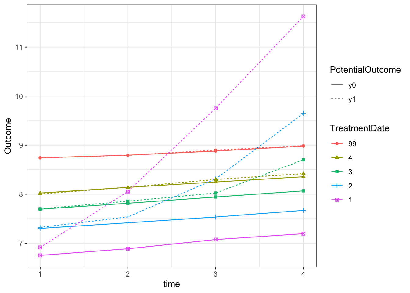

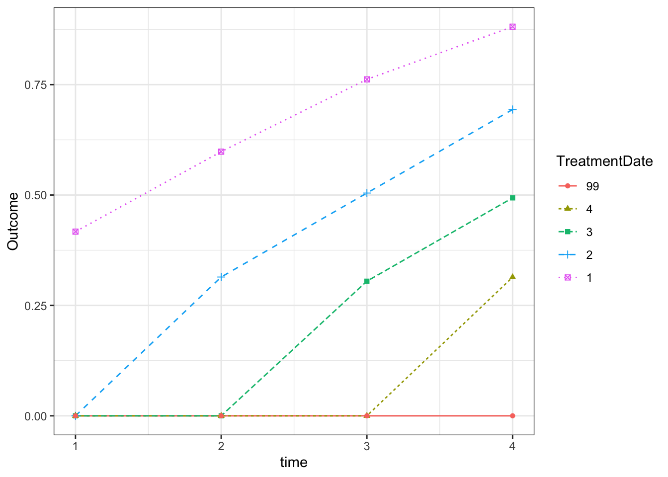
Evolution of average outcomes and treatment intensity in the various treatment groups defined by their date of entry into the treatment

Figure 4.50: Evolution of average outcomes and treatment intensity in the various treatment groups defined by their date of entry into the treatment

One final dimension of the data is how much treatment intensity varies across time and by cohort:

ggplot(data %>% filter(D>0),aes(x=treatment,color=as.factor(Ds)))+
      geom_density() +
    theme_bw() +
  xlab('TreatmentIntensity')+
  scale_color_discrete(name="TreatmentDate")+
  facet_wrap(.~time)

Figure 4.51: Distribution of treatment intensity in the various treatment groups over time

ggplot(data %>% filter(D>0,id<=30),aes(x=time,y=treatment,color=as.factor(id)))+
      geom_line() +
    theme_bw() +
  xlab('TreatmentIntensity')

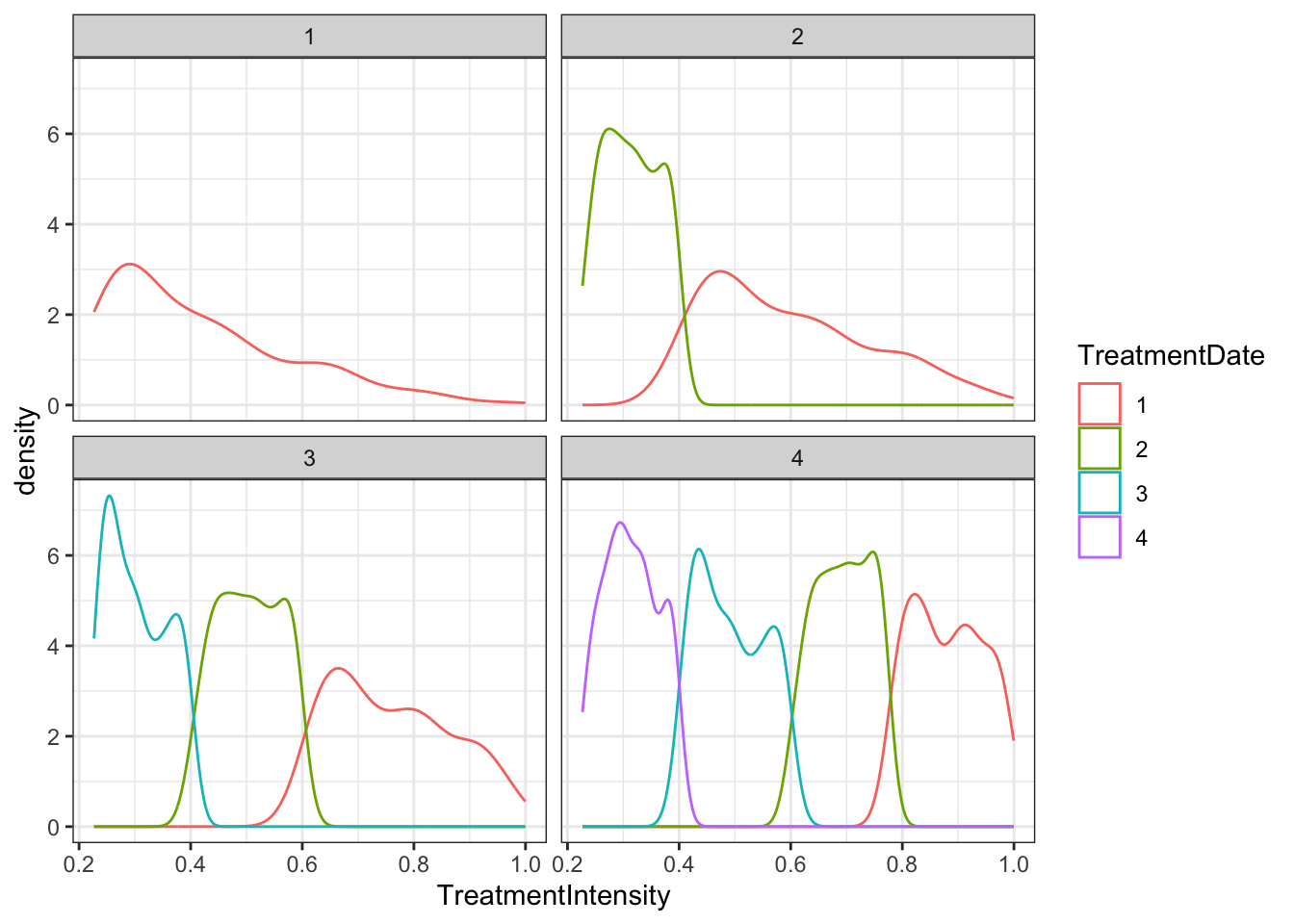
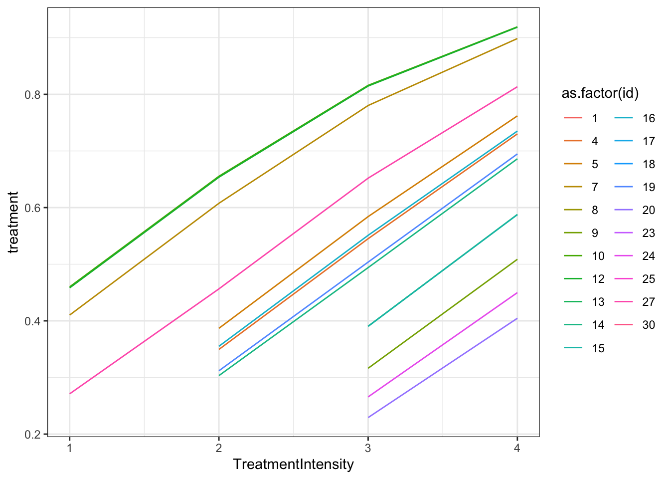
Figure 4.52: Distribution of treatment intensity in the various treatment groups over time

  #scale_color_discrete(name="TreatmentDate")+
  #facet_wrap(.~time)

As we can see on Figure ??, the model imposes that treatment intensity increases over time, which is compatible with Assumption 4.39. In practice, de Chaisemartin and d’Haultfoeuille suggest to discard observation with crossing treatment intensities over time.

4.3.5.2.1 Estimation using de Chaisemartin and d’Haultfoeuille package

Let us now try to use de Chaisemartin and d’Haultfoeuille’s did_multiplegt_dyn to estimate our treatment effects.

reg.Continuous.Staggered.DID <- did_multiplegt_dyn(df=data %>% filter(Ds>1),outcome="y",group="id",time="time",treatment="treatment",effects=3,placebo=2,graph_off=TRUE)
reg.Continuous.Staggered.DID.normalized <- did_multiplegt_dyn(df=data %>% filter(Ds>1),outcome="y",group="id",time="time",treatment="treatment",effects=3,placebo=2,graph_off=TRUE,normalized=TRUE)

We can now plot the result of the estimation of the non normalized and normalized coefficients:

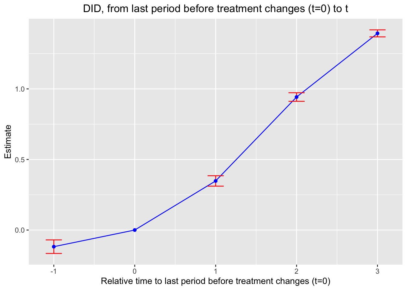
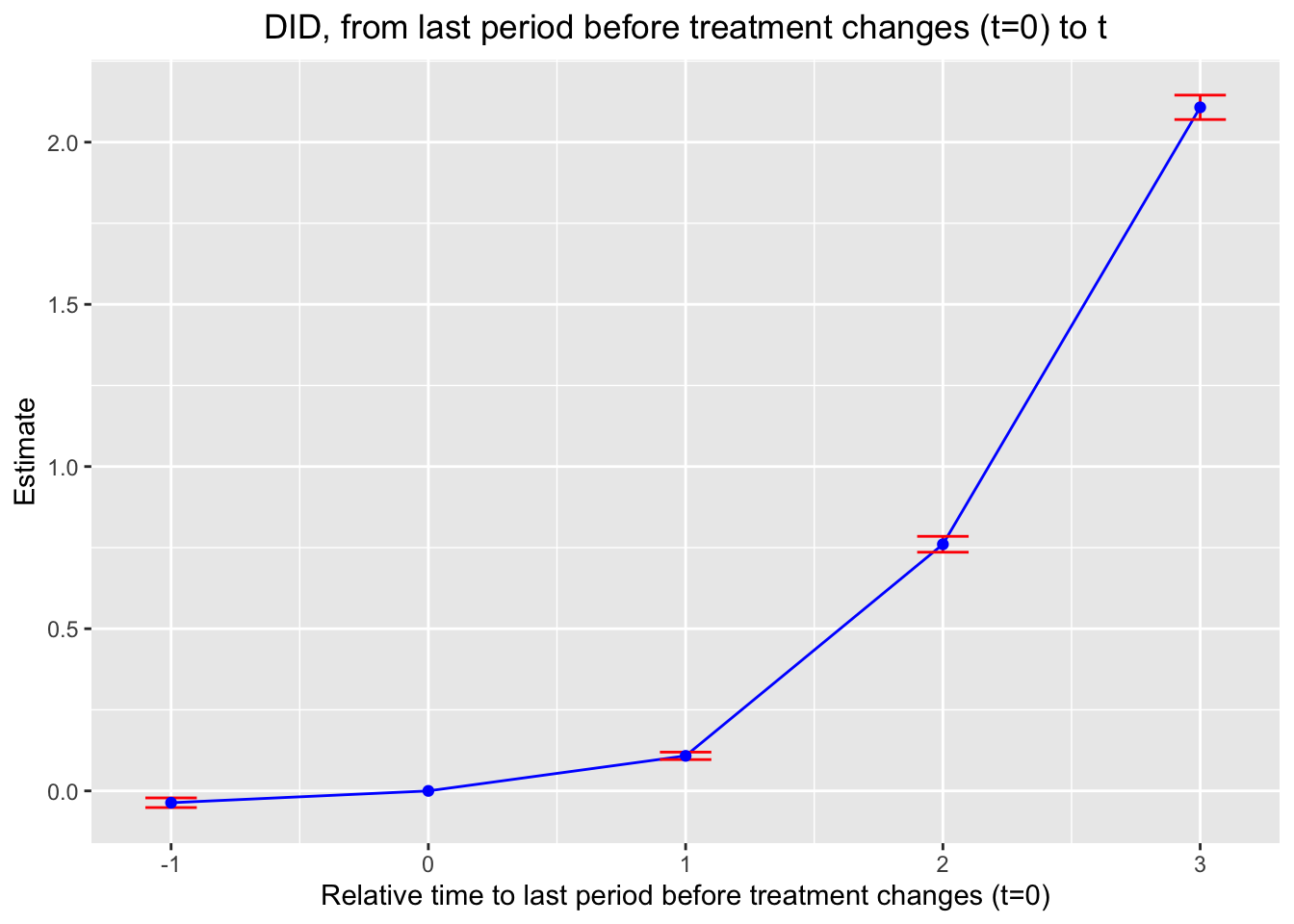
reg.Continuous.Staggered.DID.normalized$plot
reg.Continuous.Staggered.DID$plot

Figure 4.53: Estimated normalized and non-normalized treatment effects using de Chaisemartin and dHaultfoeuille estimator

Remark. Note that the estimation procedure refuses to give more than one placebo estimate, whereas two are actually feasible with this dataset.

4.3.5.2.2 Estimation using a grouped stacked first difference estimator

An alternative approach would be to identify similar treatment trajectories and estimate the treatment effects separately for each of them. One way to do that would be to use a stacked first difference estimator with groups. One way to build the groups would be to use $k$-means clustering to select sets of individuals that have very similar trajectories, enforcing for example that they have the same treatment date.

4.3.5.3 Estimation of sampling noise

One final difficulty appears when estimating the precision of the $DID_{g,l}$ estimator used in Theorem 4.36. If there is only one observation per treatment group $g$, then it is impossible to estimate heteroskedasticity robust standard errors, since the residual of the treated observation is always going to be zero. One way around this is to use the stacked first difference estimator with several observations per treatment group. But this solution requires that we assume independence between the observations in the same treatment group, which we generally are not willing to do, especially when, like here, the treatment is clustered at the group level. An alternative approach, explored by de Chaisemartin and d’Haultfoeuille, is to identify groups with similar values of the treatment dynamics, and to assume that they have very similar variances, and are mutually independent from each other. This categorization of the treatment histories is simply a way to specify the shape of heteroskedasticity in the model.