Chapter 1 Fundamental Problem of Causal Inference
In order to state the FPCI, we are going to describe the basic language to encode causality set up by Rubin, and named Rubin Causal Model (RCM). RCM being about partly observed random variables, it is hard to make these notions concrete with real data. That’s why we are going to use simulations from a simple model in order to make it clear how these variables are generated. The second virtue of this model is that it is going to make it clear the source of selection into the treatment. This is going to be useful when understanding biases of intuitive comparisons, but also to discuss the methods of causal inference. A third virtue of this approach is that it makes clear the connexion between the treatment effects literature and models. Finally, a fourth reason that it is useful is that it is going to give us a source of sampling variation that we are going to use to visualize and explore the properties of our estimators.
I use \(X_i\) to denote random variable \(X\) all along the notes. I assume that we have access to a sample of \(N\) observations indexed by \(i\in\left\{1,\dots,N\right\}\). ’‘\(i\)’’ will denote the basic sampling units when we are in a sample, and a basic element of the probability space when we are in populations. Introducing rigorous measure-theoretic notations for the population is feasible but is not necessary for comprehension.
When the sample size is infinite, we say that we have a population. A population is a very useful fiction for two reasons. First, in a population, there is no sampling noise: we observe an infinite amount of observations, and our estimators are infinitely precise. This is useful to study phenomena independently of sampling noise. For example, it is in general easier to prove that an estimator is equal to \(TT\) under some conditions in the population. Second, we are most of the time much more interested in estimating the values of parameters in the population rather than in the sample. The population parameter, independent of sampling noise, gives a much better idea of the causal parameter for the population of interest than the parameter in the sample. In general, the estimator for both quantities will be the same, but the estimators for the effetc of sampling noise on these estimators will differ. Sampling noise for the population parameter will generally be larger, since it is affected by another source of variability (sample choice).
1.1 Rubin Causal Model
RCM is made of three distinct building blocks: a treatment allocation rule, that decides who receives the treatment; potential outcomes, that measure how each individual reacts to the treatment; the switching equation that relates potential outcomes to observed outcomes through the allocation rule.
1.1.1 Treatment allocation rule
The first building block of RCM is the treatment allocation rule. Throughout this class, we are going to be interested in inferring the causal effect of only one treatment with respect to a control condition. Extensions to multi-valued treatments are in general self-explanatory.
In RCM, treatment allocation is captured by the variable \(D_i\). \(D_i=1\) if unit \(i\) receives the treatment and \(D_i=0\) if unit \(i\) does not receive the treatment and thus remains in the control condition.
The treatment allocation rule is critical for several reasons. First, because it switches the treatment on or off for each unit, it is going to be at the source of the FPCI. Second, the specific properties of the treatment allocatoin rule are going to matter for the feasibility and bias of the various econometric methods that we are going to study.
Let’s take a few examples of allocation rules. These allocation rules are just examples. They do not cover the space of all possible allocation rules. They are especially useful as concrete devices to understand the sources of biases and the nature of the allocation rule. In reality, there exists even more complex allocation rules (awareness, eligibility, application, acceptance, active participation). Awareness seems especially important for program participation and has only been tackled recently by economists.
First, some notation. Let’s imagine a treatment that is given to individuals. Whether each individual receives the treatment partly depends on the level of her outcome before receiving the treatment. Let’s denote this variable \(Y^B_i\), with \(B\) standing for “Before”. It can be the health status assessed by a professional before deciding to give a drug to a patient. It can be the poverty level of a household used to assess its eligibilty to a cash transfer program.
1.1.1.1 Sharp cutoff rule
The sharp cutoff rule means that everyone below some threshold \(\bar{Y}\) is going to receive the treatment. Everyone whose outcome before the treatment lies above \(\bar{Y}\) does not receive the treatment. Such rules can be found in reality in a lot of situations. They might be generated by administrative rules. One very simple way to model this rule is as follows:
\[\begin{align}\label{eq:cutoff} D_i & = \uns{Y_i^B\leq\bar{Y}}, \end{align}\]
where \(\uns{A}\) is the indicator function, taking value \(1\) when \(A\) is true and \(0\) otherwise.
Example 1.1 (Sharp cutoff rule) Imagine that \(Y_i^B=\exp(y_i^B)\), with \(y_i^B=\mu_i+U_i^B\), \(\mu_i\sim\mathcal{N}(\bar{\mu},\sigma^2_{\mu})\) and \(U_i^B\sim\mathcal{N}(0,\sigma^2_{U})\). Now, let’s choose some values for these parameters so that we can generate a sample of individuals and allocate the treatment among them. I’m going to switch to R for that.
##    barmu sigma2mu  sigma2U     barY
##     8.00     0.50     0.28  1500.00
Now, I have choosen values for the parameters in my model. For example, \(\bar{\mu}=\) 8 and \(\bar{Y}=\) 1500. What remains to be done is to generate \(Y_i^B\) and then \(D_i\). For this, I have to choose a sample size (\(N=1000\)) and then generate the shocks from a normal.
# for reproducibility, I choose a seed that will give me the same random sample each time I run the program
set.seed(1234)
N <-1000
mu <- rnorm(N,param["barmu"],sqrt(param["sigma2mu"]))
UB <- rnorm(N,0,sqrt(param["sigma2U"]))
yB <- mu + UB
YB <- exp(yB)
Ds <- ifelse(YB<=param["barY"],1,0)
Let’s now build a histogram of the data that we have just generated.
# building histogram of yB with cutoff point at ybar
# Number of steps
Nsteps.1 <- 15
#step width
step.1 <- (log(param["barY"])-min(yB[Ds==1]))/Nsteps.1
Nsteps.0 <- (-log(param["barY"])+max(yB[Ds==0]))/step.1
breaks <- cumsum(c(min(yB[Ds==1]),c(rep(step.1,Nsteps.1+Nsteps.0+1))))
hist(yB,breaks=breaks,main="")
abline(v=log(param["barY"]),col="red")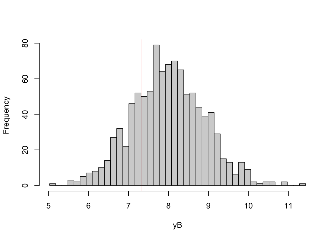
Figure 1.1: Histogram of \(y_B\)
You can see on Figure 1.1 a histogram of \(y_i^B\) with the red line indicating the cutoff point: \(\bar{y}=\ln(\bar{Y})=\) 7.3. All the observations below the red line are treated according to the sharp rule while all the one located above are not. In order to see how many observations eventually receive the treatment with this allocation rule, let’s build a contingency table.
table.D.sharp <- as.matrix(table(Ds))
knitr::kable(table.D.sharp,caption='Treatment allocation with sharp cutoff rule',booktabs=TRUE)| 0 | 771 |
| 1 | 229 |
We can see on Table 1.1 that there are 229 treated observations.
1.1.1.2 Fuzzy cutoff rule
This rule is less sharp than the sharp cutoff rule. Here, other criteria than \(Y_i^B\) enter into the decision to allocate the treatment. The doctor might measure the health status of a patient following official guidelines, but he might also measure other factors that will also influence his decision of giving the drug to the patient. The officials administering a program might measure the official income level of a household, but they might also consider other features of the household situation when deciding to enroll the household into the program or not. If these additional criteria are unobserved to the econometrician, then we have the fuzzy cutoff rule. A very simple way to model this rule is as follows:
\[\begin{align}\label{eq:fuzzcutoff} D_i & = \uns{Y_i^B+V_i\leq\bar{Y}}, \end{align}\]
where \(V_i\) is a random variable unobserved to the econometrician and standing for the other influences that might drive the allocation of the treatment. \(V_i\) is distributed according to a, for the moment, unspecified cumulative distribution function \(F_V\). When \(V_i\) is degenerate ( it has only one point of support: it is a constant), the fuzzy cutoff rule becomes the sharp cutoff rule.
1.1.1.3 Eligibility \(+\) self-selection rule
It is also possible that households, once they have been made eligible to the treatment, can decide whether they want to receive it or not. A patient might be able to refuse the drug that the doctor suggests she should take. A household might refuse to participate in a cash transfer program to which it has been made eligible. Not all programs have this feature, but most of them have some room for decisions by the agents themselves of whether they want to receive the treatment or not. One simple way to model this rule is as follows:
\[\begin{align}\label{eq:eligself} D_i & = \uns{D^*_i\geq0}E_i, \end{align}\]
where \(D^*_i\) is individual \(i\)’s valuation of the treatment and \(E_i\) is whether or not she is deemed eligible for the treatment. \(E_i\) might be choosen according to the sharp cutoff rule of to the fuzzy cutoff rule, or to any other eligibility rule. We will be more explicit about \(D_i^*\) in what follows.
SIMULATIONS ARE MISSING FOR THESE LAST TWO RULES
1.1.2 Potential outcomes
The second main building block of RCM are potential outcomes. Let’s say that we are interested in the effect of a treatment on an outcome \(Y\). Each unit \(i\) can thus be in two potential states: treated or non treated. Before the allocation of the treatment is decided, both of these states are feasible for each unit.
Definition 1.1 (Potential outcomes) For each unit \(i\), we define two potential outcomes:
- \(Y_i^1\): the outcome that unit \(i\) is going to have if it receives the treatment,
- \(Y_i^0\): the outcome that unit \(i\) is going to have if it does not receive the treatment.
Example 1.2 Let’s choose functional forms for our potential outcomes. For simplicity, all lower case letters will denote log outcomes. \(y_i^0=\mu_i+\delta+U_i^0\), with \(\delta\) a time shock common to all the observations and \(U_i^0=\rho U_i^B+\epsilon_i\), with \(|\rho|<1\). In the absence of the treatment, part of the shocks \(U_i^B\) that the individuals experienced in the previous period persist, while some part vanish. \(y_i^1=y_i^0+\bar{\alpha}+\theta\mu_i+\eta_i\). In order to generate the potential outcomes, one has to define the laws for the shocks and to choose parameter values. Let’s assume that \(\epsilon_i\sim\mathcal{N}(0,\sigma^2_{\epsilon})\) and \(\eta_i\sim\mathcal{N}(0,\sigma^2_{\eta})\). Now let’s choose some parameter values:
l <- length(param)
param <- c(param,0.9,0.01,0.05,0.05,0.05,0.1)
names(param)[(l+1):length(param)] <- c("rho","theta","sigma2epsilon","sigma2eta","delta","baralpha")
param
## barmu sigma2mu sigma2U barY rho
## 8.00 0.50 0.28 1500.00 0.90
## theta sigma2epsilon sigma2eta delta baralpha
## 0.01 0.05 0.05 0.05 0.10We can finally generate the potential outcomes;
epsilon <- rnorm(N,0,sqrt(param["sigma2epsilon"]))
eta<- rnorm(N,0,sqrt(param["sigma2eta"]))
U0 <- param["rho"]*UB + epsilon
y0 <- mu +  U0 + param["delta"]
alpha <- param["baralpha"]+  param["theta"]*mu + eta
y1 <- y0+alpha
Y0 <- exp(y0)
Y1 <- exp(y1)
Now, I would like to visualize my potential outcomes:
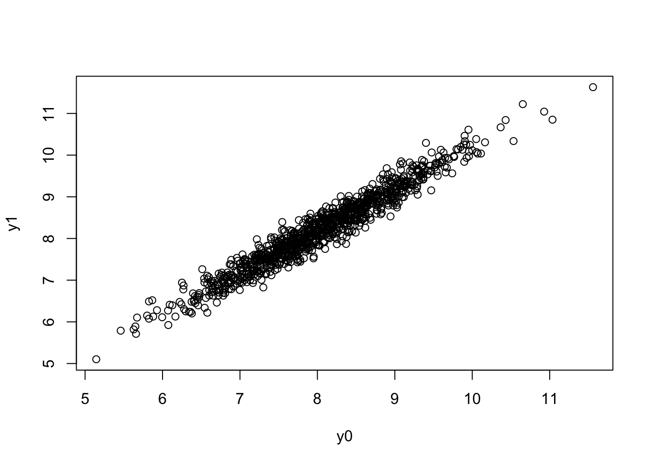
Figure 1.2: Potential outcomes
You can see on the resulting Figure 1.2 that both potential outcomes are positively correlated. Those with a large potential outcome when untreated (e.g. in good health without the treatment) also have a positive health with the treatment. It is also true that individuals with bad health in the absence of the treatment also have bad health with the treatment.
1.1.3 Switching equation
The last building block of RCM is the switching equation. It links the observed outcome to the potential outcomes through the allocation rule:
\[\begin{align} \tag{1.1} Y_i & = \begin{cases} Y_i^1 & \text{if } D_i=1\\ Y_i^0 & \text{if } D_i=0 \end{cases} \\ & = Y_i^1D_i + Y_i^0(1-D_i) \nonumber \end{align}\]
Example 1.3 In order to generate observed outcomes in our numerical example, we simply have to enforce the switching equation:
What the switching equation (1.1) means is that, for each individual \(i\), we get to observe only one of the two potential outcomes. When individual \(i\) belongs to the treatment group (i.e. \(D_i=1\)), we get to observe \(Y_i^1\). When individual \(i\) belongs to the control group (i.e. \(D_i=0\)), we get to observe \(Y_i^0\). Because the same individual cannot be at the same time in both groups, we can NEVER see both potential outcomes for the same individual at the same time.
For each of the individuals, one of the two potential outcomes is unobserved. We say that it is a counterfactual. A counterfactual quantity is a quantity that is, according to Hume’s definition, contrary to the observed facts. A counterfactual cannot be observed, but it can be conceived by an effort of reason: it is the consequence of what would have happened had some action not been taken.
Remark. One very nice way of visualising the switching equation has been proposed by Jerzy Neyman in a 1923 prescient paper. Neyman proposes to imagine two urns, each one filled with \(N\) balls. One urn is the treatment urn and contains balls with the id of the unit and the value of its potential outcome \(Y_i^1\). The other urn is the control urn, and it contains balls with the value of the potential outcome \(Y_i^0\) for each unit \(i\). Following the allocation rule \(D_i\), we decide whether unit \(i\) is in the treatment or control group. When unit \(i\) is in the treatment group, we take the corresponding ball from the first urn and observe the potential outcome on it. But, at the same time, the urns are connected so that the corresponding ball with the potential outcome of unit \(i\) in the control urn disappears as soon as we draw ball \(i\) from the treatment urn.
The switching equation works a lot like Schrodinger’s cat paradox. Schrodinger’s cat is placed in a sealed box and receives a dose of poison when an atom emits a radiation. As long as the box is sealed, there is no way we can know whether the cat is dead or alive. When we open the box, we observe either a dead cat or a living cat, but we cannot observe the cat both alive and dead at the same time. The switching equation is like opening the box, it collapses the observed outcome into one of the two potential ones.
Example 1.4 One way to visualize the inner workings of the switching equation is to plot the potential outcomes along with the criteria driving the allocation rule. In our simple example, it simply amounts to plotting observed (\(y_i\)) and potential outcomes (\(y_i^1\) and \(y_i^0\)) along \(y_i^B\).
plot(yB[Ds==0],y0[Ds==0],pch=1,xlim=c(5,11),ylim=c(5,11),xlab="yB",ylab="Outcomes")
points(yB[Ds==1],y1[Ds==1],pch=3)
points(yB[Ds==0],y1[Ds==0],pch=3,col='red')
points(yB[Ds==1],y0[Ds==1],pch=1,col='red')
test <- 5.8
i.test <- which(abs(yB-test)==min(abs(yB-test)))
points(yB[abs(yB-test)==min(abs(yB-test))],y1[abs(yB-test)==min(abs(yB-test))],col='green',pch=3)
points(yB[abs(yB-test)==min(abs(yB-test))],y0[abs(yB-test)==min(abs(yB-test))],col='green')
abline(v=log(param["barY"]),col="red")
legend(5,11,c('y0|D=0','y1|D=1','y0|D=1','y1|D=0',paste('y0',i.test,sep=''),paste('y1',i.test,sep='')),pch=c(1,3,1,3,1,3),col=c('black','black','red','red','green','green'),ncol=3)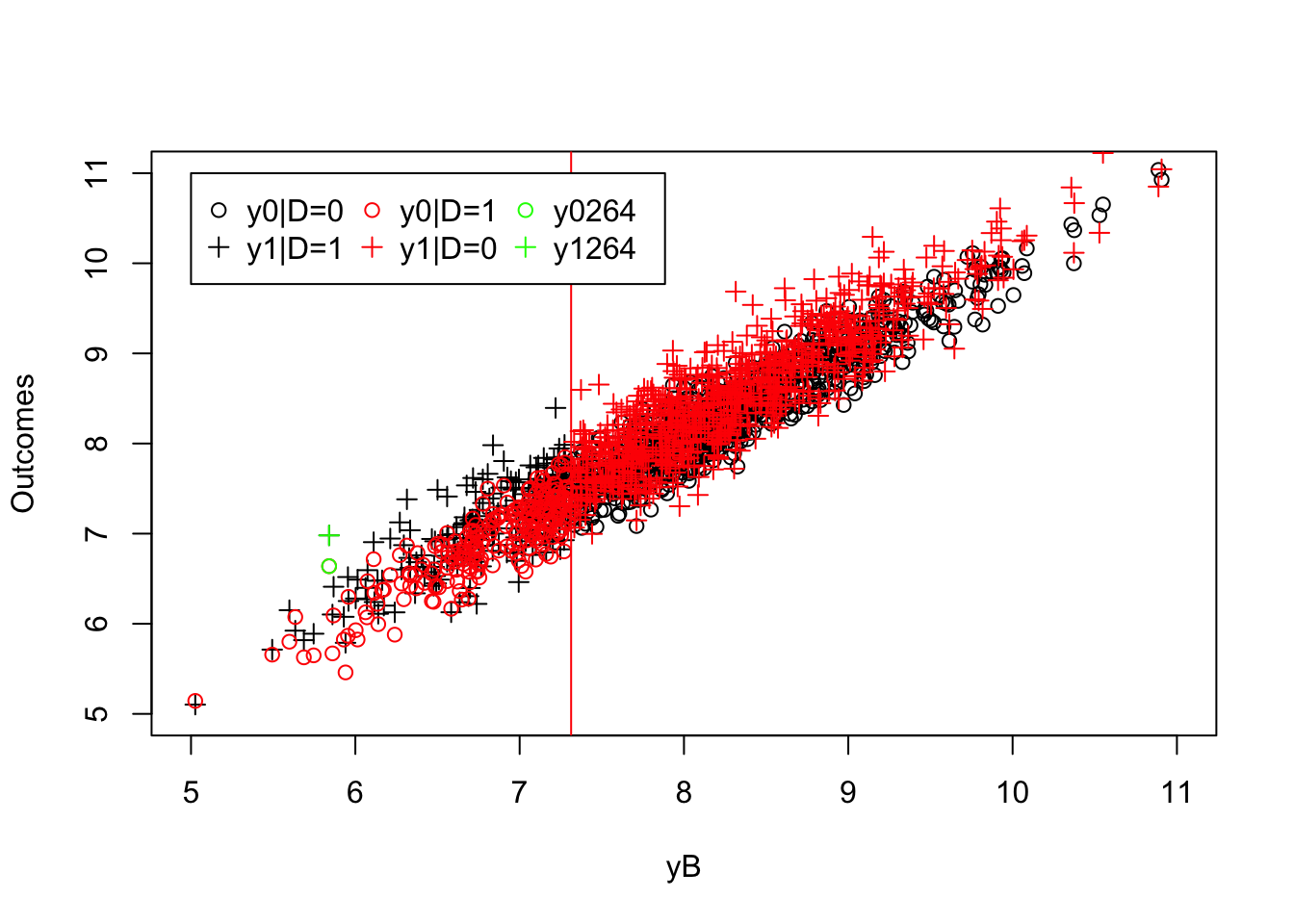
Figure 1.3: Potential outcomes
plot(yB[Ds==0],y0[Ds==0],pch=1,xlim=c(5,11),ylim=c(5,11),xlab="yB",ylab="Outcomes")
points(yB[Ds==1],y1[Ds==1],pch=3)
legend(5,11,c('y|D=0','y|D=1'),pch=c(1,3))
abline(v=log(param["barY"]),col="red")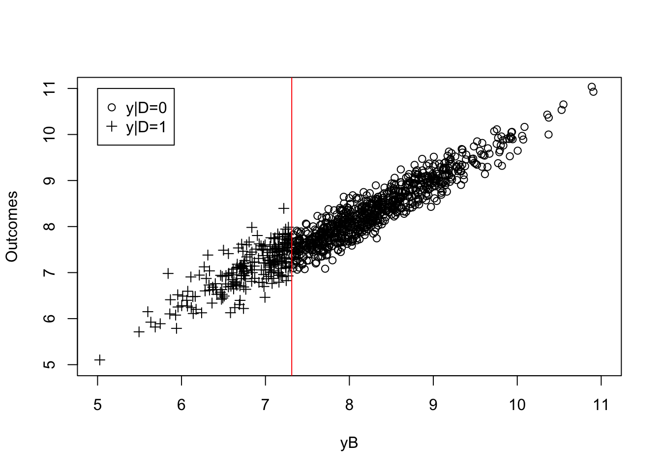
Figure 1.4: Observed outcomes
Figure 1.3 plots the observed outcomes \(y_i\) along with the unobserved potential outcomes. Figure 1.3 shows that each individual in the sample is endowed with two potential outcomes, represented by a circle and a cross. Figure 1.4 plots the observed outcomes \(y_i\) that results from applying the switching equation. Only one of the two potential outcomes is observed (the cross for the treated group and the circle for the untreated group) and the other is not. The observed sample in Figure 1.4 only shows observed outcomes, and is thus silent on the values of the missing potential outcomes.
1.2 Treatment effects
RCM enables the definition of causal effects at the individual level. In practice though, we generally focus on a summary measure: the effect of the treatment on the treated.
1.2.1 Individual level treatment effects
Potential outcomes enable us to define the central notion of causal inference: the causal effect, also labelled the treatment effect, which is the difference between the two potential outcomes.
Definition 1.2 (Individual level treatment effect) For each unit \(i\), the causal effect of the treatment on outcome \(Y\) is: \(\Delta^Y_i=Y_i^1-Y_i^0\).
Example 1.5 The individual level causal effect in log terms is: \(\Delta^y_i=\alpha_i=\bar{\alpha}+\theta\mu_i+\eta_i\). The effect is the sum of a part common to all individuals, a part correlated with \(\mu_i\): the treatment might have a larger or a smaller effect depending on the unobserved permanent ability or health status of individuals, and a random shock. It is possible to make the effect of the treatment to depend on \(U_i^B\) also, but it would complicate the model.
In Figure 1.3, the individual level treatment effects are the differences between each cross and its corresponding circle. For example, for observation 264, the two potential outcomes appear in green in Figure 1.3. The effect of the treatment on unit 264 is equal to: \[ \Delta^y_{264}=y^1_{264}-y^0_{264}=6.98-6.64=0.34. \]
Since observation 264 belongs to the treatment group, we can only observe the potential outcome in the presence of the treatment, \(y^1_{264}\).
RCM allows for heterogeneity of treatment effects. The treatment has a large effect on some units and a much smaller effect on other units. We can even have some units that benefit from the treatment and some units that are harmed by the treatment. The individual level effect of the treatment is itself a random variable (and not a fixed parameter). It has a distribution, \(F_{\Delta^Y}\).
Heterogeneity of treatment effects seems very natural: the treatment might interact with individuals’ different backgrounds. The effect of a drug might depend on the genetic background of an individual. An education program might only work for children that already have sufficient non-cognitive skills, and thus might depend in turn on family background. An environmental regulation or a behavioral intervention might only trigger reactions by already environmentally aware individuals. A CCT might have a larger effect when indiviuals are credit-constrained or face shocks.
Example 1.6 In our numerical example, the distribution of \(\Delta^y_i=\alpha_i\) is a normal: \(\alpha_i\sim\mathcal{N}(\bar{\alpha}+\theta\bar{\mu},\theta^2\sigma^2_{\mu}+\sigma^2_{\eta})\). We would like to visualize treatment effect heterogeneity. For that, we can build a histogram of the individual level causal effect.
On top of the histogram, we can also draw the theoretical distribution of the treatment effect: a normal with mean 0.18 and variance 0.05.
hist(alpha,main="",prob=TRUE)
curve(dnorm(x, mean=(param["baralpha"]+param["theta"]*param["barmu"]), sd=sqrt(param["theta"]^2*param["sigma2mu"]+param["sigma2eta"])), add=TRUE,col='red')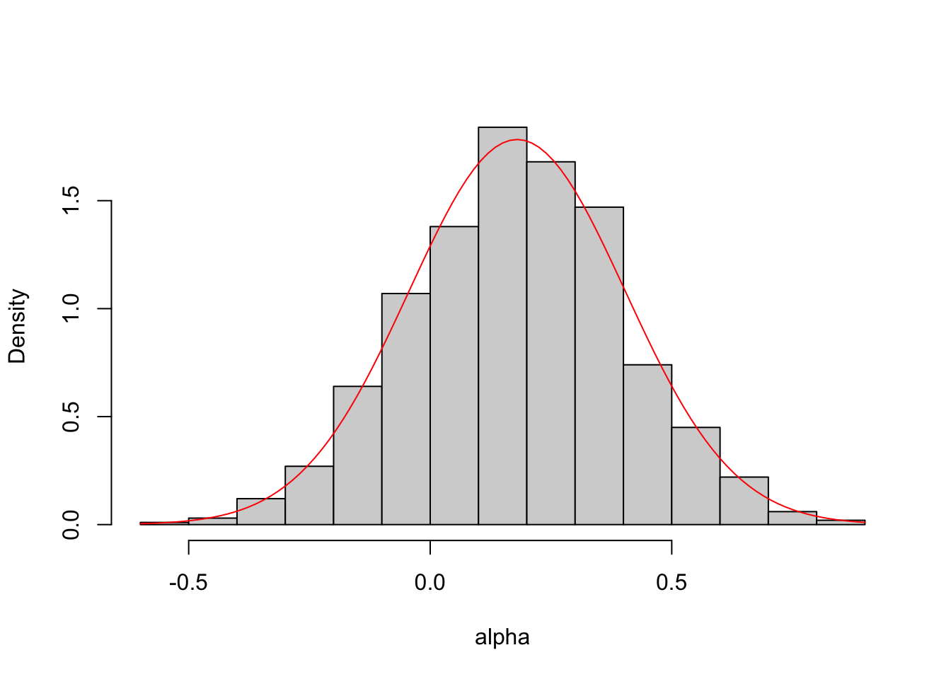
Figure 1.5: Histogram of \(\Delta^y\)
The first thing that we can see on Figure 1.5 is that the theoretical and the empirical distributions nicely align with each other. We also see that the majority of the observations lies to the right of zero: most people experience a positive effect of the treatment. But there are some individuals that do not benefit from the treatment: the effect of the treatment on them is negative.
1.2.2 Average treatment effect on the treated
We do not generally estimate individual-level treatment effects. We generally look for summary statistics of the effect of the treatment. By far the most widely reported causal parameter is the Treatment on the Treated parameter (TT). It can be defined in the sample at hand or in the population.
Definition 1.3 (Average and expected treatment effects on the treated) The Treatment on the Treated parameters for outcome \(Y\) are:
The average Treatment effect on the Treated in the sample:
\[\begin{align*} \Delta^Y_{TT_s} & = \frac{1}{\sum_{i=1}^ND_i}\sum_{i=1}^N(Y_i^1-Y_i^0)D_i, \end{align*}\]
The expected Treatment effect on the Treated in the population:
\[\begin{align*} \Delta^Y_{TT} & = \esp{Y_i^1-Y_i^0|D_i=1}. \end{align*}\]
The TT parameters measure the average effect of the treatment on those who actually take it, either in the sample at hand or in the popluation. It is generally considered to be the most policy-relevant parameter since it measures the effect of the treatment as it has actually been allocated. For example, the expected causal effect on the overall population is only relevant if policymakers are considering implementing the treatment even on those who have not been selected to receive it. For a drug or an anti-poverty program, it would mean giving the treatment to healthy or rich people, which would make little sense.
TT does not say anything about how the effect of the treatment is distributed in the population or in the sample. TT does not account for the heterogneity of treatment effects. In Lecture 7, we will look at other parameters of interest that look more closely into how the effect of the treatment is distributed.
Example 1.7 The value of TT in our sample is:
\[ \Delta^y_{TT_s}=0.168. \]
Computing the population value of \(TT\) is slightly more involved: we have to use the formula for the conditional expectation of a censored bivariate normal random variable:
\[\begin{align*} \Delta^y_{TT} & = \esp{\alpha_i|D_i=1}\\ & = \bar{\alpha}+\theta\esp{\mu_i|\mu_i+U_i^B\leq\bar{y}}\\ & = \bar{\alpha}+\theta\left(\bar{\mu} - \frac{\sigma^2_{\mu}}{\sqrt{\sigma^2_{\mu}+\sigma^2_{U}}}\frac{\phi\left(\frac{\bar{y}-\bar{\mu}}{\sqrt{\sigma^2_{\mu}+\sigma^2_{U}}}\right)}{\Phi\left(\frac{\bar{y}-\bar{\mu}}{\sqrt{\sigma^2_{\mu}+\sigma^2_{U}}}\right)}\right)\\ & = \bar{\alpha}+\theta\bar{\mu}-\theta\left(\frac{\sigma^2_{\mu}}{\sqrt{\sigma^2_{\mu}+\sigma^2_{U}}}\frac{\phi\left(\frac{\bar{y}-\bar{\mu}}{\sqrt{\sigma^2_{\mu}+\sigma^2_{U}}}\right)}{\Phi\left(\frac{\bar{y}-\bar{\mu}}{\sqrt{\sigma^2_{\mu}+\sigma^2_{U}}}\right)}\right), \end{align*}\]
where \(\phi\) and \(\Phi\) are respectively the density and the cumulative distribution functions of the standard normal. The second equality follows from the definition of \(\alpha_i\) and \(D_i\) and from the fact that \(\eta_i\) is independent from \(\mu_i\) and \(U_i^B\). The third equality comes from the formula for the expectation of a censored bivariate normal random variable. In order to compute the population value of TT easily for different sets of parameter values, let’s write a function in R:
delta.y.tt <- function(param){return(param["baralpha"]+param["theta"]*param["barmu"]
-param["theta"]*((param["sigma2mu"]*dnorm((log(param["barY"])-param["barmu"])/(sqrt(param["sigma2mu"]+param["sigma2U"]))))
/(sqrt(param["sigma2mu"]+param["sigma2U"])
*pnorm((log(param["barY"])-param["barmu"])/(sqrt(param["sigma2mu"]+param["sigma2U"]))))))}The population value of TT computed using this function is: \(\Delta^y_{TT}=\) 0.172. We can see that the values of TT in the sample and in the population differ slightly. This is because of sampling noise: the units in the sample are not perfectly representative of the units in the population.
1.3 Fundamental problem of causal inference
At least in this lecture, causal inference is about trying to infer TT, either in the sample or in the population. The FPCI states that it is impossible to directly observe TT because one part of it remains fundamentally unobserved.
Theorem 1.1 (Fundamental problem of causal inference) It is impossible to observe TT, either in the population or in the sample.
Proof. The proof of the FPCI is rather straightforward. Let me start with the sample TT:
\[\begin{align*} \Delta^Y_{TT_s} & = \frac{1}{\sum_{i=1}^ND_i}\sum_{i=1}^N(Y_i^1-Y_i^0)D_i \\ & = \frac{1}{\sum_{i=1}^ND_i}\sum_{i=1}^NY_i^1D_i- \frac{1}{\sum_{i=1}^ND_i}\sum_{i=1}^NY_i^0D_i \\ & = \frac{1}{\sum_{i=1}^ND_i}\sum_{i=1}^NY_iD_i- \frac{1}{\sum_{i=1}^ND_i}\sum_{i=1}^NY_i^0D_i. \end{align*}\]
Since \(Y_i^0\) is unobserved whenever \(D_i=1\), \(\frac{1}{\sum_{i=1}^ND_i}\sum_{i=1}^NY_i^0D_i\) is unobserved, and so is \(\Delta^Y_{TT_s}\). The same is true for the population TT:
\[\begin{align*} \Delta^Y_{TT} & = \esp{Y_i^1-Y_i^0|D_i=1} \\ & = \esp{Y_i^1|D_i=1}-\esp{Y_i^0|D_i=1}\\ & = \esp{Y_i|D_i=1}-\esp{Y_i^0|D_i=1}. \end{align*}\]
\(\esp{Y_i^0|D_i=1}\) is unobserved, and so is \(\Delta^Y_{TT}\).
The key insight in order to understand the FPCI is to see that the outcomes of the treated units had they not been treated are unobservable, and so is their average or expectation. We say that they are counterfactual, contrary to what has happened.
Definition 1.4 (Couterfactual) Both \(\frac{1}{\sum_{i=1}^ND_i}\sum_{i=1}^NY_i^0D_i\) and \(\esp{Y_i^0|D_i=1}\) are counterfactual quantities that we will never get to observe.
Example 1.8 The average counterfactual outcome of the treated is the mean of the red circles in the \(y\) axis on Figure 1.3:
\[ \frac{1}{\sum_{i=1}^ND_i}\sum_{i=1}^Ny_i^0D_i= 6.91. \] Remember that we can estimate this quantity only because we have generated the data ourselves. In real life, this quantity is hopelessly unobserved.
\(\esp{y_i^0|D_i=1}\) can be computed using the formula for the expectation of a censored normal random variable:
\[\begin{align*} \esp{y_i^0|D_i=1} & = \esp{\mu_i+\delta+U_i^0|D_i=1}\\ & = \esp{\mu_i+\delta+\rho U_i^B+\epsilon_i|D_i=1}\\ & = \delta + \esp{\mu_i+\rho U_i^B|y_i^B\leq\bar{y}}\\ & = \delta + \bar{\mu} - \frac{\sigma^2_{\mu}+\rho\sigma^2_U}{\sqrt{\sigma^2_{\mu}+\sigma^2_{U}}}\frac{\phi\left(\frac{\bar{y}-\bar{\mu}}{\sqrt{\sigma^2_{\mu}+\sigma^2_{U}}}\right)}{\Phi\left(\frac{\bar{y}-\bar{\mu}}{\sqrt{\sigma^2_{\mu}+\sigma^2_{U}}}\right)}. \end{align*}\]
We can write a function in R to compute this value:
esp.y0.D1 <- function(param){
return(param["delta"]+param["barmu"]
-((param["sigma2mu"]+param["rho"]*param["sigma2U"])
*dnorm((log(param["barY"])-param["barmu"])/(sqrt(param["sigma2mu"]+param["sigma2U"]))))
/(sqrt(param["sigma2mu"]+param["sigma2U"])*pnorm((log(param["barY"])-param["barmu"])
/(sqrt(param["sigma2mu"]+param["sigma2U"])))))
}The population value of TT computed using this function is: \(\esp{y_i^0|D_i=1}=\) 6.9.
1.4 Intuitive estimators, confounding factors and selection bias
In this section, we are going to examine the properties of two intuitive comparisons that laypeople, policymakers but also ourselves make in order to estimate causal effects: the with/wihtout comparison (\(WW\)) and the before/after comparison (\(BA\)). \(WW\) compares the average outcomes of the treated individuals with those of the untreated individuals. \(BA\) compares the average outcomes of the treated after taking the treatment to their average outcomes before they took the treatment. These comparisons try to proxy for the expected counterfactual outcome in the treated group by using an observed quantity. \(WW\) uses the expected outcome of the untreated individuals as a proxy. \(BA\) uses the expected outcome of the treated before they take the treatment as a proxy.
Unfortunately, both of these proxies are generally poor and provide biased estimates of \(TT\). The reason that these proxies are poor is that the treatment is not the only factor that differentiates the treated group from the groups used to form the proxy. The intuitive comparisons are biased because factors, other than the treatment, are correlated to its allocation. The factors that bias the intuitive comparisons are generally called confouding factors or confounders.
The treatment effect measures the effect of a ceteris paribus change in treatment status, while the intuitive comparisons capture both the effect of this change and that of other correlated changes that spuriously contaminate the comparison. Intuitive comparisons measure correlations while treatment effects measure causality. The old motto “correlation is not causation” applies vehemently here.
Remark. A funny anecdote about this expression “correlation is not causation”. This expression is due to Karl Pearson, the father of modern statistics. He coined the phrase in his famous book “The Grammar of Science.” Pearson is famous for inventing the correlation coefficient. He actually thought that correlation was a much superior, much more rigorous term, than causation. In his book, he actually used the sentence to argue in favor of abandoning causation altogether and focusing on the much better-defined and measurable concept of correlation. Interesting turn of events that his sentence is now used to mean that correlation is weaker than causation, totally reverting the original intended meaning.
In this section, we are going to define both comparisons, study their biases and state the conditions under which they identify \(TT\). This will prove to be a very useful introduction to the notion of identification. It is also very important to be able to understand the sources of bias of comparisons that we use every day and that come very naturally to policy makers and lay people.
Remark. In this section, we state the definitions and formulae in the population. This is for two reasons. First, it is simpler, and lighter in terms of notation. Second, it emphasizes that the problems with intuitive comparisons are independent of sampling noise. Most of the results stated here for the population extend to the sample, replacing the expectation operator by the average operator. I will nevertheless give examples in the sample, since it is so much simpler to compute. I will denote sample equivalents of population estimators with a hat.
1.4.1 With/Without comparison, selection bias and cross-sectional confounders
The with/without comparison (\(WW\)) is very intuitive: just compare the outcomes of the treated and untreated individuals in order to estimate the causal effect. This approach is nevertheless generally biased. We call the bias of \(WW\) selection bias (\(SB\)). Selection bias is due to unobserved confounders that are distributed differently in the treatment and control group and that generate differences in outcomes even in the absence of the treatment. In this section, I define the \(WW\) estimator, derives its bias, introduces the confounders and states conditions under which it is unbiased.
1.4.1.1 With/Without comparison
The with/without comparison (\(WW\)) is very intuitive: just compare the outcomes of the treated and untreated individuals in order to estimate the causal effect.
Definition 1.5 (With/without comparison) The with/without comparison is the difference between the expected outcomes of the treated and the expected outcomes of the untreated:
\[\begin{align*} \Delta^Y_{WW} & = \esp{Y_i|D_i=1}-\esp{Y_i|D_i=0}. \end{align*}\]
Example 1.9 In the population, \(WW\) can be computed using the traditional formula for the expectation of a truncated normal distribution:
\[\begin{align*} \Delta^y_{WW} & = \esp{y_i|D_i=1}-\esp{y_i|D_i=0} \\ & = \esp{y_i^1|D_i=1}-\esp{y^0_i|D_i=0} \\ & = \esp{\alpha_i|D_i=1}+\esp{\mu_i+\rho U_i^B|\mu_i+U_i^B\leq\bar{y}}-\esp{\mu_i+\rho U_i^B|\mu_i+U_i^B>\bar{y}} \\ & = \bar{\alpha}+\theta\left(\bar{\mu}-\frac{\sigma^2_{\mu}}{\sqrt{\sigma^2_{\mu}+\sigma^2_{U}}}\frac{\phi\left(\frac{\bar{y}-\bar{\mu}}{\sqrt{\sigma^2_{\mu}+\sigma^2_{U}}}\right)}{\Phi\left(\frac{\bar{y}-\bar{\mu}}{\sqrt{\sigma^2_{\mu}+\sigma^2_{U}}}\right)}\right) -\frac{\sigma^2_{\mu}+\rho\sigma^2_{U}}{\sqrt{\sigma^2_{\mu}+\sigma^2_{U}}}\left(\frac{\phi\left(\frac{\bar{y}-\bar{\mu}}{\sqrt{\sigma^2_{\mu}+\sigma^2_{U}}}\right)}{\Phi\left(\frac{\bar{y}-\bar{\mu}}{\sqrt{\sigma^2_{\mu}+\sigma^2_{U}}}\right)}+\frac{\phi\left(\frac{\bar{y}-\bar{\mu}}{\sqrt{\sigma^2_{\mu}+\sigma^2_{U}}}\right)}{1-\Phi\left(\frac{\bar{y}-\bar{\mu}}{\sqrt{\sigma^2_{\mu}+\sigma^2_{U}}}\right)}\right). \end{align*}\]
In order to compute this parameter, we are going to set up a R function. For reasons that will become clearer later, we will define two separate functions to compute the first and second part of the formula. In the first part, you should have recognised \(TT\), that we have already computed in Lecture 1. We are going to call the second part \(SB\), for reasons that will become explicit in a bit.
delta.y.tt <- function(param){
return(param["baralpha"]+param["theta"]*param["barmu"]-param["theta"]
*((param["sigma2mu"]*dnorm((log(param["barY"])-param["barmu"])
/(sqrt(param["sigma2mu"]+param["sigma2U"]))))
/(sqrt(param["sigma2mu"]+param["sigma2U"])*pnorm((log(param["barY"])-param["barmu"])
/(sqrt(param["sigma2mu"]+param["sigma2U"]))))))
}
delta.y.sb <- function(param){
return(-(param["sigma2mu"]+param["rho"]*param["sigma2U"])/sqrt(param["sigma2mu"]+param["sigma2U"])
*dnorm((log(param["barY"])-param["barmu"])/(sqrt(param["sigma2mu"]+param["sigma2U"])))
*(1/pnorm((log(param["barY"])-param["barmu"])/(sqrt(param["sigma2mu"]+param["sigma2U"])))
+1/(1-pnorm((log(param["barY"])-param["barmu"])/(sqrt(param["sigma2mu"]+param["sigma2U"]))))))
}
delta.y.ww <- function(param){
return(delta.y.tt(param)+delta.y.sb(param))
}As a conclusion of all these derivations, \(WW\) in the population is equal to -1.298. Remember that the value of \(TT\) in the population is 0.172.
In order to compute the \(WW\) estimator in a sample, I’m going to generate a brand new sample and I’m going to choose a seed for the pseudo-random number generator so that we obtain the same result each time we run the code.
I use set.seed(1234) in the code chunk below.
param <- c(8,.5,.28,1500)
names(param) <- c("barmu","sigma2mu","sigma2U","barY")
set.seed(1234)
N <-1000
mu <- rnorm(N,param["barmu"],sqrt(param["sigma2mu"]))
UB <- rnorm(N,0,sqrt(param["sigma2U"]))
yB <- mu + UB
YB <- exp(yB)
Ds <- rep(0,N)
Ds[YB<=param["barY"]] <- 1
l <- length(param)
param <- c(param,0.9,0.01,0.05,0.05,0.05,0.1)
names(param)[(l+1):length(param)] <- c("rho","theta","sigma2epsilon","sigma2eta","delta","baralpha")
epsilon <- rnorm(N,0,sqrt(param["sigma2epsilon"]))
eta<- rnorm(N,0,sqrt(param["sigma2eta"]))
U0 <- param["rho"]*UB + epsilon
y0 <- mu + U0 + param["delta"]
alpha <- param["baralpha"]+ param["theta"]*mu + eta
y1 <- y0+alpha
Y0 <- exp(y0)
Y1 <- exp(y1)
y <- y1*Ds+y0*(1-Ds)
Y <- Y1*Ds+Y0*(1-Ds)In this sample, the average outcome of the treated in the presence of the treatment is \[ \frac{1}{\sum_{i=1}^ND_i}\sum_{i=1}^ND_iy_i= 7.074. \] It is materialized by a circle on Figure 1.6. The average outcome of the untreated is \[ \frac{1}{\sum_{i=1}^N(1-D_i)}\sum_{i=1}^N(1-D_i)y_i= 8.383. \] It is materialized by a plus sign on Figure 1.6.
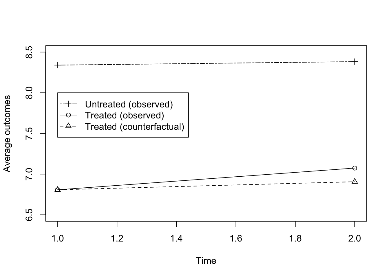
Figure 1.6: Evolution of average outcomes in the treated and control group before (Time =1) and after (Time=2) the treatment
The estimate of the \(WW\) comparison in the sample is thus:
\[\begin{align*} \hat{\Delta^Y_{WW}} & = \frac{1}{\sum_{i=1}^N D_i}\sum_{i=1}^N Y_iD_i-\frac{1}{\sum_{i=1}^N (1-D_i)}\sum_{i=1}^N Y_i(1-D_i). \end{align*}\]
We have \(\hat{\Delta^y_{WW}}=\) -1.308. Remember that the value of \(TT\) in the sample is \(\Delta^y_{TT_s}=\) 0.168.
Overall, \(WW\) severely underestimates the effect of the treatment in our example. \(WW\) suggests that the treatment has a negative effect on outcomes whereas we know by construction that it has a positive one.
1.4.1.2 Selection bias
When we form the with/without comparison, we do not recover the \(TT\) parameter. Instead, we recover \(TT\) plus a bias term, called selection bias:
\[\begin{align*} \Delta^Y_{WW} & =\Delta^Y_{TT}+\Delta^Y_{SB}. \end{align*}\]
Definition 1.6 (Selection bias) Selection bias is the difference between the with/without comparison and the treatment on the treated parameter: \[\begin{align*} \Delta^Y_{SB} & = \Delta^Y_{WW}-\Delta^Y_{TT}. \end{align*}\]
\(WW\) tries to approximate the counterfactual expected outcome in the treated group by using \(\esp{Y_i^0|D_i=0}\), the expected outcome in the untreated group . Selection bias appears because this proxy is generally poor. It is very easy to see that selection bias is indeed directly due to this bad proxy problem:
Theorem 1.2 (Selection bias and counterfactual) Selection bias is the difference between the counterfactual expected potential outcome in the absence of the treatment among the treated and the expected potential outcome in the absence of the treatment among the untreated.
\[\begin{align*} \Delta^Y_{SB} & = \esp{Y_i^0|D_i=1}-\esp{Y_i^0|D_i=0}. \end{align*}\]
Proof. \[\begin{align*} \Delta^Y_{SB} & = \Delta^Y_{WW}-\Delta^Y_{TT} \\ & = \esp{Y_i|D_i=1}-\esp{Y_i|D_i=0}-\esp{Y_i^1-Y_i^0|D_i=1}\\ & = \esp{Y_i^0|D_i=1}-\esp{Y_i^0|D_i=0}. \end{align*}\]
The first and second equalities stem only from the definition of both parameters. The third equality stems from using the switching equation: \(Y_i=Y_i^1D_i+Y_i^0(1-D_i)\), so that \(\esp{Y_i|D_i=1}=\esp{Y^1_i|D_i=1}\) and \(\esp{Y_i|D_i=0}=\esp{Y_i^0|D_i=0}\).
Example 1.10 In the population, \(SB\) is equal to
\[\begin{align*} \Delta^y_{SB} & = \Delta^y_{WW}-\Delta^y_{TT} \\ & = -1.298 - 0.172 \\ & = -1.471 \end{align*}\]
We could have computed \(SB\) directly using the formula from Theorem 1.2:
\[\begin{align*} \Delta^y_{SB} & = \esp{y_i^0|D_i=1}-\esp{y_i^0|D_i=0}\\ & = -\frac{\sigma^2_{\mu}+\rho\sigma^2_{U}}{\sqrt{\sigma^2_{\mu}+\sigma^2_{U}}}\left(\frac{\phi\left(\frac{\bar{y}-\bar{\mu}}{\sqrt{\sigma^2_{\mu}+\sigma^2_{U}}}\right)}{\Phi\left(\frac{\bar{y}-\bar{\mu}}{\sqrt{\sigma^2_{\mu}+\sigma^2_{U}}}\right)}+\frac{\phi\left(\frac{\bar{y}-\bar{\mu}}{\sqrt{\sigma^2_{\mu}+\sigma^2_{U}}}\right)}{1-\Phi\left(\frac{\bar{y}-\bar{\mu}}{\sqrt{\sigma^2_{\mu}+\sigma^2_{U}}}\right)}\right). \end{align*}\]
When using the R function for \(SB\) that we have defined earlier, we indeed find: \(\Delta^y_{SB}=\) -1.471.
In the sample, \(\hat{\Delta^y_{SB}}=\)-1.308-0.168 \(=\) -1.476. Selection bias emerges because we are using a bad proxy for the counterfactual. The average outcome for the untreated is equal to \(\frac{1}{\sum_{i=1}^N(1-D_i)}\sum_{i=1}^N(1-D_i)y_i=\) 8.383 while the counterfactual average outcome for the treated is \(\frac{1}{\sum_{i=1}^ND_i}\sum_{i=1}^ND_iy^0_i=\) 6.906. Their difference is as expected equal to \(SB\): \(\hat{\Delta^y_{SB}}=\) 6.906 \(-\) 8.383 \(=\) -1.476. The counterfactual average outcome of the treated is much smaller than the average outcome of the untreated. On Figure 1.6, this is materialized by the fact that the plus sign is located much above the triangle.
Remark. The concept of selection bias is related to but different from the concept of sample selection bias. With sample selection bias, we worry that selection into the sample might bias the estimated effect of a treatment on outcomes. With selection bias, we worry that selection into the treatment itself might bias the effect of the treatment on outcomes. Both biases are due to unbserved covariates, but they do not play out in the same way.
For example, estimating the effect of education on women’s wages raises both selection bias and sample selection bias issues. Selection bias stems from the fact that more educated women are more likely to be more dynamic and thus to have higher earnings even when less educated. Selection bias would be positive in that case, overestimating the effect of education on earnings.
Sample selection bias stems from the fact that we can only use a sample of working women in order to estimate the effect of education on wages, since we do not observe the wages on non working women. But, selection into the labor force might generate sample selection bias. More educated women participate more in the labor market, while less educated women participate less. As a consequence, less educated women that work are different from the overall sample of less educated women. They might be more dynamic and work-focused. As a consequence, their wages are higher than the average wages of the less educated women. Comparing the wages of less educated women that work to those of more educated women that work might understate the effect of education on earnings. Sample selection bias would generate a negative bias on the education coefficient.
1.4.1.3 Confounding factors
Confounding factors are the factors that generate differences between treated and untreated individuals even in the absence of the treatment. The confounding factors are thus responsible for selection bias. In general, the mere fact of being selected for receiving the treatment means that you have a host of characteristics that would differentiate you from the unselected individuals, even if you were not to receive the treatment eventually.
For example, if a drug is given to initially sicker individuals, then, we expect that they will be sicker that the untreated in the absence of the treatment. Comparing sick individuals to healthy ones is not a sound way to estimate the effect of a treatment. Obviously, even if our treatment performs well, healthier individuals will be healthier after the treatment has been allocated to the sicker patients. The best we can expect is that the treated patients have recovered, and that their health after the treatment is comparable to that of the untreated patients. In that case, the with/without comparison is going to be null, whereas the true effect of the treatment is positive. Selection bias is negative in that case: in the absence of the treatment, the average health status of the treated individuals would have been smaller than that of the untreated individuals. The confounding factor is the health status of individuals when the decision to allocate the drug has been taken. It is correlated to both the allocation of the treatment (negatively) and to health in the absence of the treatment (positively).
Example 1.11 In our example, \(\mu_i\) and \(U_i^B\) are the confounding factors. Because the treatment is only given to individuals with pre-treament outcomes smaller than a threshold (\(y_i^B\leq\bar{y}\)), participants tend to have smaller \(\mu_i\) and \(U_i^B\) than non participants, as we can see on Figure 1.7.
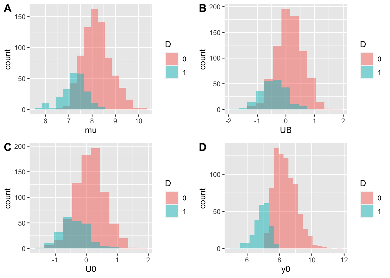
Figure 1.7: Distribution of confounders in the treated and control group
Since confounding factors are persistent, they affect the outcomes of participants and non participants after the treatment date. \(\mu_i\) persists entirely over time, and \(U_i^B\) persists at a rate \(\rho\). As a consequence, even in the absence of the treatment, participants have lower outcomes than non participants, as we can see on Figure 1.7.
We can derive the contributions of both confouding factors to overall SB:
\[\begin{align*} \esp{Y_i^0|D_i=1} & = \esp{\mu_i+\delta+U_i^0|\mu_i+U_i^B\leq\bar{y}}\\ & = \delta + \esp{\mu_i|\mu_i+U_i^B\leq\bar{y}} + \rho\esp{U_i^B|\mu_i+U_i^B\leq\bar{y}}\\ \Delta^y_{SB} & = \esp{\mu_i|\mu_i+U_i^B\leq\bar{y}}-\esp{\mu_i|\mu_i+U_i^B>\bar{y}} \\ & \phantom{=} + \rho\left(\esp{U_i^B|\mu_i+U_i^B\leq\bar{y}}-\esp{U_i^B|\mu_i+U_i^B>\bar{y}}\right)\\ & = -\frac{\sigma^2_{\mu}}{\sqrt{\sigma^2_{\mu}+\sigma^2_{U}}}\left(\frac{\phi\left(\frac{\bar{y}-\bar{\mu}}{\sqrt{\sigma^2_{\mu}+\sigma^2_{U}}}\right)}{\Phi\left(\frac{\bar{y}-\bar{\mu}}{\sqrt{\sigma^2_{\mu}+\sigma^2_{U}}}\right)}+\frac{\phi\left(\frac{\bar{y}-\bar{\mu}}{\sqrt{\sigma^2_{\mu}+\sigma^2_{U}}}\right)}{1-\Phi\left(\frac{\bar{y}-\bar{\mu}}{\sqrt{\sigma^2_{\mu}+\sigma^2_{U}}}\right)}\right) \\ & \phantom{=} -\frac{\rho\sigma^2_{U}}{\sqrt{\sigma^2_{\mu}+\sigma^2_{U}}}\left(\frac{\phi\left(\frac{\bar{y}-\bar{\mu}}{\sqrt{\sigma^2_{\mu}+\sigma^2_{U}}}\right)}{\Phi\left(\frac{\bar{y}-\bar{\mu}}{\sqrt{\sigma^2_{\mu}+\sigma^2_{U}}}\right)}+\frac{\phi\left(\frac{\bar{y}-\bar{\mu}}{\sqrt{\sigma^2_{\mu}+\sigma^2_{U}}}\right)}{1-\Phi\left(\frac{\bar{y}-\bar{\mu}}{\sqrt{\sigma^2_{\mu}+\sigma^2_{U}}}\right)}\right) \end{align*}\]
In order to evaluate these quantities, let’s build two R functions:
delta.y.sb.mu <- function(param){
return(-(param["sigma2mu"])/sqrt(param["sigma2mu"]+param["sigma2U"])
*dnorm((log(param["barY"])-param["barmu"])/(sqrt(param["sigma2mu"]+param["sigma2U"])))
*(1/pnorm((log(param["barY"])-param["barmu"])/(sqrt(param["sigma2mu"]+param["sigma2U"])))
+1/(1-pnorm((log(param["barY"])-param["barmu"])/(sqrt(param["sigma2mu"]+param["sigma2U"]))))))
}
delta.y.sb.U <- function(param){
return(-(param["rho"]*param["sigma2U"])/sqrt(param["sigma2mu"]+param["sigma2U"])
*dnorm((log(param["barY"])-param["barmu"])/(sqrt(param["sigma2mu"]+param["sigma2U"])))
*(1/pnorm((log(param["barY"])-param["barmu"])/(sqrt(param["sigma2mu"]+param["sigma2U"])))
+1/(1-pnorm((log(param["barY"])-param["barmu"])/(sqrt(param["sigma2mu"]+param["sigma2U"]))))))
}The contribution of \(\mu_i\) to selection bias is -0.978 while that of \(U_i^0\) is of -0.493.
1.4.1.4 When does \(WW\) identify \(TT\)?
Are there conditions under which \(WW\) identify \(TT\)? The answer is yes: when there is no selection bias, the proxy used by \(WW\) for the counterfactual quantity is actually valid. Formally, \(WW\) identifies \(TT\) when the following assumption holds:
Definition 1.7 (No selection bias) We assume the following: \[\begin{align*} \esp{Y_i^0|D_i=1} & = \esp{Y_i^0|D_i=0}. \end{align*}\]
Under Assumption 1.7, the expected counterfactual outcome of the treated is equal to the expected potential outcome of the untreated in the absence of the treatment. This yields to the following result:
Theorem 1.3 Under Assumption 1.7, \(WW\) identifies the \(TT\) parameter: \[\begin{align*} \Delta^Y_{WW} & = \Delta^Y_{TT}. \end{align*}\]
Proof. \[\begin{align*} \Delta^Y_{WW} & = \esp{Y_i|D_i=1}-\esp{Y_i|D_i=0}\\ & = \esp{Y_i^1|D_i=1}-\esp{Y_i^0|D_i=0}\\ & = \esp{Y_i^1|D_i=1}-\esp{Y_i^0|D_i=1} \\ & = \Delta^Y_{TT}, \end{align*}\] where the second equation uses the switching equation and the third uses Assumption 1.7.
So, under Assumption 1.7, the \(WW\) comparison actually identifies the \(TT\) parameter. We say that Assumption 1.7 is an identification assumption: it serves to identify the parameter of interest using observed data. The intuition for this result is simply that, under Assumption 1.7, there are no confounding factors and thus no selection bias. under Assumption 1.7, the factors that yield individuals to receive or not the treatment are mean-independent of the potential outcomes in the absence of the treatment. In this case, the expected outcome in the untreated group actually is a perfect proxy for the counterfactual expected outcome of the treated group.
Obviously, Assumption 1.7 is extremely unlikely to hold in real life. For Assumption 1.7 to hold, it has to be that all the determinants of \(D_i\) are actually unrelated to \(Y_i^0\). One way to enforce Assumption 1.7 is to randomize treatment intake. We will see this in the Lecture on RCTs. It might also be possible that Assumption 1.7 holds in the data in the absence of an RCT. But this is not very likely, and should be checked by every mean possible.
One way to test for the validity of Assumption 1.7 is to compare the values of observed covariates in the treated and untreated group. For Assumption 1.7 to be credible, observed covariates should be distributed in the same way.
Another nice way to test for the validity of Assumption 1.7 with observed data is to implement a placebo test. A placebo test looks for an effect where there should be none, if we believe the identification assumptions. For example, under Assumption 1.7 it should be (even though it is not rigorously implied) that outcomes before the treatment are also mean-independent of the treatment allocation. And actually, since a future treatment cannot have an effect today (unless people anticipate the treatment, which we assume away here), the \(WW\) comparison before the treatment should be null, therefore giving a zero effect of the placebo treatment “will receive the treatment in the future.”
Example 1.12 When the allocation rule defining \(D_i\) is the eligibility rule that we have used so far, we have already seen that Assumption 1.7 does not hold and the placebo test should not pass either.
One way of generating Assumption 1.7 from the eligibility rule that we are using is to mute the persistence in outcome dynamics. For example, one could set \(\rho=0\) and \(\sigma^2_{\mu}=0\).
param <- c(8,0,.28,1500,0,0.01,0.05,0.05,0.05,0.1)
names(param) <- c("barmu","sigma2mu","sigma2U","barY","rho","theta","sigma2epsilon","sigma2eta","delta","baralpha")
param## barmu sigma2mu sigma2U barY rho
## 8.00 0.00 0.28 1500.00 0.00
## theta sigma2epsilon sigma2eta delta baralpha
## 0.01 0.05 0.05 0.05 0.10In that case, outcomes are not persistent and Assumption 1.7 holds:
\[\begin{align*} \esp{y_i^0|D_i=1} & = \esp{\mu_i+\delta+U_i^0|y_i^B\leq\bar{y}}\\ & = \esp{\bar{\mu}+\delta+\epsilon_i|\bar{\mu}+U_i^B\leq\bar{y}}\\ & = \bar{\mu} + \delta + \esp{\epsilon_i|\bar{\mu}+U_i^B\leq\bar{y}}\\ & = \bar{\mu} + \delta + \esp{\epsilon_i|\bar{\mu}+U_i^B>\bar{y}}\\ & = \esp{\mu_i+\delta+U_i^0|y_i^B>\bar{y}}\\ & = \esp{y_i^0|D_i=0}, \end{align*}\]
where the second equality follows from \(\sigma^2_{\mu}=0\) and \(\rho=0\) and the fourth from \(\epsilon_i \Ind U_i^B\). Another direct way to see this is to use the formula for selection bias that we have derived above. It is easy to see that with \(\rho=0\) and \(\sigma^2_{\mu}=0\), \(\Delta^y_{SB}=0\). To be sure, we can compute \(\Delta^y_{SB}\) with the new parameter values: \(\Delta^y_{SB}=\) 0. As a consequence, \(\Delta^y_{TT}=\) 0.18 \(=\) 0.18 \(=\Delta^y_{WW}\).
Remark. You might have noticed that the value of \(\Delta^y_{TT}\) is different than before. It is normal, since it depends on the values of parameters, and especially on \(\sigma_{\mu}^2\) and \(\rho\).
Let’s see how these quantities behave in the sample.
set.seed(1234)
mu <- rnorm(N,param["barmu"],sqrt(param["sigma2mu"]))
UB <- rnorm(N,0,sqrt(param["sigma2U"]))
yB <- mu + UB
YB <- exp(yB)
Ds <- rep(0,N)
Ds[YB<=param["barY"]] <- 1
epsilon <- rnorm(N,0,sqrt(param["sigma2epsilon"]))
eta<- rnorm(N,0,sqrt(param["sigma2eta"]))
U0 <- param["rho"]*UB + epsilon
y0 <- mu + U0 + param["delta"]
alpha <- param["baralpha"]+ param["theta"]*mu + eta
y1 <- y0+alpha
Y0 <- exp(y0)
Y1 <- exp(y1)
y <- y1*Ds+y0*(1-Ds)
Y <- Y1*Ds+Y0*(1-Ds)We can see that \(\hat{\esp{Y_i^0|D_i=1}}=\) 8.038 \(\approx\) 8.055 \(=\hat{\esp{Y_i^0|D_i=0}}\). This means that \(WW\) should be close to \(TT\): \(\hat{\Delta^y_{TT}}=\) 0.198 \(\approx\) 0.182 \(=\hat{\Delta^y_{WW}}\). Note that \(\hat{WW}\) in the sample is not exactly, but only approximately, equal to \(TT\) in the population and in the sample. This is an instance of the Fundamental Problem of Statistical Inference that we will study in the next chapter.
Under these restrictions, the placebo test would unfortunately conclude against Assumption 1.7 even though it is valid:
\[\begin{align*} \esp{y_i^B|D_i=1} & = \esp{\mu_i+ U_i^B|y_i^B\leq\bar{y}}\\ & = \esp{\bar{\mu}+U_i^B|\bar{\mu}+U_i^B\leq\bar{y}}\\ & = \bar{\mu} + \esp{U_i^B|\bar{\mu}+U_i^B\leq\bar{y}}\\ & \neq \bar{\mu} + \esp{U_i^B|\bar{\mu}+U_i^B>\bar{y}}\\ & = \esp{\mu_i+U_i^0|y_i^B>\bar{y}}\\ & = \esp{y_i^B|D_i=0}. \end{align*}\]
In the sample, we indeed have that \(\hat{\esp{Y_i^B|D_i=1}}=\) 7.004 \(\neq\) 8.072 \(=\hat{\esp{Y_i^B|D_i=0}}\). The reason for the failure of the placebo test to conclude that \(Ww\) is actually correct is that the \(U_i^B\) shock enters both into the selection equation and the outcome equation for \(y_i^B\), generating a wage at period \(B\) between the outcomes of the treated and of the untreated. Since it is not persistent, this wedge does not generate selection bias. This wedge would not be detected if we could perform it further back in time, before the selection period.
Another way to make Assumption 1.7 work is to generate a new allocation rule where all the determinants of treatment intake are indeed orthogonal to potential outcomes and to outcomes before the treatment. Let’s assume for example that \(D_i=\uns{V_i\leq\bar{y}}\), with \(V_i\sim\mathcal{N}(\bar{\mu},\sigma^2_{\mu}+\sigma^2_{U})\) and \(V_i\Ind(Y_i^0,Y_i^1,Y_i^B,\mu_i,\eta_i)\). In that case, Assumption 1.7 holds and the placebo test does work. Indeed, we have:
\[\begin{align*} \Delta^y_{TT} & = \esp{Y_i^1-Y_i^0|D_i=1} \\ & = \esp{\alpha_i|D_i=1} \\ & = \esp{\bar{\alpha}+\theta\mu_i+\eta_i|V_i\leq\bar{y}}\\ & = \bar{\alpha}+\theta\bar{\mu} \\ & = \Delta^y_{ATE} \\ \Delta^y_{WW} & = \esp{Y_i|D_i=1} - \esp{Y_i|D_i=0} \\ & = \esp{Y^1_i|D_i=1} - \esp{Y^0_i|D_i=0} \\ & = \esp{Y^1_i|V_i\leq\bar{y}} - \esp{Y^0_i|V_i>\bar{y}} \\ & = \esp{Y^1_i} - \esp{Y^0_i} \\ & = \Delta^y_{ATE} \end{align*}\]
\(ATE\) is the Average Treatment Effect in the population. It is the expected effect of the treatment on all the members of the population, not only on the treated. When the treatment is randomly allocated, both \(TT\) and \(ATE\) are equal, since the treated are a random subset of the overall population. I prefer to use \(ATE\) for my definition of the \(R\) function in order not to erase the definition of the \(TT\) function:
In the population, \(WW\) identifies \(TT\): \(\Delta^y_{TT}=\) 0.18 \(=\Delta^y_{WW}\). Let’s see how these quantities behave in the sample:
set.seed(1234)
N <-1000
mu <- rnorm(N,param["barmu"],sqrt(param["sigma2mu"]))
UB <- rnorm(N,0,sqrt(param["sigma2U"]))
yB <- mu + UB
YB <- exp(yB)
Ds <- rep(0,N)
V <- rnorm(N,param["barmu"],sqrt(param["sigma2mu"]+param["sigma2U"]))
Ds[V<=log(param["barY"])] <- 1
epsilon <- rnorm(N,0,sqrt(param["sigma2epsilon"]))
eta<- rnorm(N,0,sqrt(param["sigma2eta"]))
U0 <- param["rho"]*UB + epsilon
y0 <- mu + U0 + param["delta"]
alpha <- param["baralpha"]+ param["theta"]*mu + eta
y1 <- y0+alpha
Y0 <- exp(y0)
Y1 <- exp(y1)
y <- y1*Ds+y0*(1-Ds)
Y <- Y1*Ds+Y0*(1-Ds)In the sample, the counterfactual is well approximated by the outcomes of the untreated: \(\hat{\esp{Y_i^0|D_i=1}}=\) 8.085 \(\approx\) 8.054 \(=\hat{\esp{Y_i^0|D_i=0}}\). As a consequence, \(WW\) should be close to \(TT\): \(\hat{\Delta^y_{TT}}=\) 0.168 \(\approx\) 0.199 \(=\hat{\Delta^y_{WW}}\). The placebo test is also valid in that case: \(\hat{\esp{Y_i^B|D_i=1}}=\) 7.95 \(\approx\) 7.99 \(=\hat{\esp{Y_i^B|D_i=0}}\).
1.4.2 The before/after comparison, temporal confounders and time trend bias
The before/after comparison (\(BA\)) is also very intuitive: it consists in looking at how the outcomes of the treated have changed over time and to attribute this change to the effect of the treatment. The problem is that other changes might have affected outcomes in the absence of the treatment, thereby biasing \(BA\). The bias of \(BA\) is called time-trend bias. It is due to confounders that affect the outcomes of the treated over time. This section defines the \(BA\) estimator, derives its bias, describes the role of the confounders and states conditions under which \(BA\) identifies \(TT\).
Example 1.13 Before computing any estimates, we need to reset all our parameter values and generated sample it their usual values:
param <- c(8,.5,.28,1500)
names(param) <- c("barmu","sigma2mu","sigma2U","barY")
set.seed(1234)
N <-1000
mu <- rnorm(N,param["barmu"],sqrt(param["sigma2mu"]))
UB <- rnorm(N,0,sqrt(param["sigma2U"]))
yB <- mu + UB
YB <- exp(yB)
Ds <- rep(0,N)
Ds[YB<=param["barY"]] <- 1
l <- length(param)
param <- c(param,0.9,0.01,0.05,0.05,0.05,0.1)
names(param)[(l+1):length(param)] <- c("rho","theta","sigma2epsilon","sigma2eta","delta","baralpha")
epsilon <- rnorm(N,0,sqrt(param["sigma2epsilon"]))
eta<- rnorm(N,0,sqrt(param["sigma2eta"]))
U0 <- param["rho"]*UB + epsilon
y0 <- mu +  U0 + param["delta"]
alpha <- param["baralpha"]+  param["theta"]*mu + eta
y1 <- y0+alpha
Y0 <- exp(y0)
Y1 <- exp(y1)
y <- y1*Ds+y0*(1-Ds)
Y <- Y1*Ds+Y0*(1-Ds)1.4.2.1 The before/after comparison
The before/after estimator (\(BA\)) compares the outcomes of the treated after taking the treatment to the outcomes of the treated before taking the treatment. It is also sometimes called a “pre-post comparison.”
Definition 1.8 (Before/after comparison) The before/after comparison is the difference between the expected outcomes in the treated group after the treatment and the expected outcomes in the same group before the treatment: \[\begin{align*} \Delta^Y_{BA} & = \esp{Y_i|D_i=1}-\esp{Y^B_i|D_i=1}. \end{align*}\]
Example 1.14 In the population, the \(BA\) estimator has the following shape: \[\begin{align*} \Delta^y_{BA} & = \esp{y_i|D_i=1}-\esp{y^B_i|D_i=1}\\ & = \esp{y^1_i-y^B_i|D_i=1}\\ & = \esp{\alpha_i|D_i=1} + \delta + (\rho-1)\esp{U_i^B|\mu_i+U_i^B\leq\bar{y}}\\ & = \Delta^y_{TT} + \delta + (1-\rho)\left(\frac{\sigma^2_{U}}{\sqrt{\sigma^2_{\mu}+\sigma^2_{U}}}\frac{\phi\left(\frac{\bar{y}-\bar{\mu}}{\sqrt{\sigma^2_{\mu}+\sigma^2_{U}}}\right)}{\Phi\left(\frac{\bar{y}-\bar{\mu}}{\sqrt{\sigma^2_{\mu}+\sigma^2_{U}}}\right)}\right). \end{align*}\]
In order to compute \(BA\) in the population, we can again use a R function, combining the value of \(TT\) and that of the second part of the formula, that we are going to denote \(TB\) for reasons that are going to become clear in a bit.
delta.y.tb <- function(param){
return(param["delta"]
+(1-param["rho"])*((param["sigma2U"])/sqrt(param["sigma2mu"]+param["sigma2U"]))
*dnorm((log(param["barY"])-param["barmu"])/(sqrt(param["sigma2mu"]+param["sigma2U"])))
/pnorm((log(param["barY"])-param["barmu"])/(sqrt(param["sigma2mu"]+param["sigma2U"]))))
}
delta.y.ba <- function(param){
return(delta.y.tt(param)+ delta.y.tb(param))
}The value of \(BA\) in the population is thus \(\Delta^y_{BA}=\) 0.265. Remember that the true value of \(TT\) in the population is 0.172. In the sample, the value of \(BA\) is \(\hat{\Delta^y_{BA}}=\) 0.267. Remember that the value of \(TT\) in the sample is \(\Delta^y_{TT_s}=\) 0.168.
1.4.2.2 Time trend bias
When we form the before/after comparison, we do not recover the \(TT\) parameter. Instead, we recover \(TT\) plus a bias term, called time trend bias:
\[\begin{align*} \Delta^Y_{BA} & =\Delta^Y_{TT}+\Delta^Y_{TB}. \end{align*}\]
Definition 1.9 (Time trend bias) Time trend bias is the difference between the before/after comparison and the treatment on the treated parameter: \[\begin{align*} \Delta^Y_{TB} & = \Delta^Y_{BA}-\Delta^Y_{TT} . \end{align*}\]
\(BA\) uses the expected outcome in the treated group before the treatment as a proxy for the expected counterfactual outcome in the absence of the treatment in the same group. \(TB\) is due to the fact that \(BA\) uses an imperfect proxy for the counterfactual expected outcome of the treated:
Theorem 1.4 Time trend bias is the difference between the counterfactual expected potential outcome in the absence of the treatment among the treated and the expected outcome before the treatment in the same group. \[\begin{align*} \Delta^Y_{TB} & = \esp{Y_i^0|D_i=1}-\esp{Y_i^B|D_i=1}. \end{align*}\]
Proof. \[\begin{align*} \Delta^Y_{TB} & = \Delta^Y_{BA}-\Delta^Y_{TT} \\ & = \esp{Y_i|D_i=1}-\esp{Y^B_i|D_i=1}-\esp{Y_i^1-Y_i^0|D_i=1}\\ & = \esp{Y_i^0|D_i=1}-\esp{Y_i^B|D_i=1}. \end{align*}\] The first and second equalities stem from the definition of both parameters. The third equality stems from using the switching equation: \(Y_i=Y_i^1D_i+Y_i^0(1-D_i)\), so that \(\esp{Y_i|D_i=1}=\esp{Y^1_i|D_i=1}\).
Example 1.15 In the population, \(TB\) is equal to
\(\Delta^y_{TB}=\Delta^y_{BA}-\Delta^y_{TT}=\) 0.265 \(-\) 0.172 \(=\) 0.093. We could have computed this result using Theorem1.4:
\[\begin{align*} \Delta^y_{TB} & = \esp{y_i^0|D_i=1}-\esp{y_i^B|D_i=1} \\ & = \delta + (1-\rho)\left(\frac{\sigma^2_{U}}{\sqrt{\sigma^2_{\mu}+\sigma^2_{U}}}\frac{\phi\left(\frac{\bar{y}-\bar{\mu}}{\sqrt{\sigma^2_{\mu}+\sigma^2_{U}}}\right)}{\Phi\left(\frac{\bar{y}-\bar{\mu}}{\sqrt{\sigma^2_{\mu}+\sigma^2_{U}}}\right)}\right). \end{align*}\]
Using the R function that we have defined previously, this approach gives \(\Delta^y_{TB}=\) 0.093.
In the sample \(\hat{\Delta^y_{BA}}=\) 0.267 while \(\hat{\Delta^y_{TT}}=\) 0.168, so that \(\hat{\Delta^y_{TB}}=\) 0.099. Time trend bias emerges because we are using a bad proxy for the counterfactual average outcomes of the treated. The average outcome of the treated before the treatment takes place is \(\hat{\esp{y_i^B|D_i=1}}=\) 6.807 while the true counterfactual average outcome for the treated after the treatment is \(\hat{\esp{y_i^0|D_i=1}}=\) 6.906. Outcomes would have increased in the treatment group even in the absence of the treatment. As a consequence, the \(BA\) comparison overestimates the true effect of the treatment. \(TB\) estimated using Theorem 1.4 is equal to: \(\hat{\Delta^y_{TB}}=\) 6.906 \(-\) 6.807 \(=\) 0.099. This can be seen on Figure 1.6: the triangle in period 2 is higher than in period 1.
1.4.2.3 Temporal confounders
Temporal confounders make the outcomes of the treated change at the same time as the treatment status changes, thereby confounding the effect of the treatment. Temporal confounders are responsible for time trend bias.
Over time, there are other things that change than the treatment status. For example, maybe sick individuals naturally recover, and thus their counterfactual health status is better than ther health status before taking the treatment. As a results, \(BA\) might overstimate the effect of the treatment. It might also be that the overall level of health in the country has increased, because of increasing GDP, for example.
Example 1.16 In our example, \(\delta\) and \(U_i^B\) are the confounders. \(\delta\) captures the overall changes in outcomes over time (business cycle, general improvement of health status). \(U^B_i\) captures the fact that transitorily sicker individuals tend at the same time to receive the treatment and also to recover naturally. The \(BA\) comparison incorrectly attributes both of these changes to the effect of the treatment. We can compute the relative contributions of both sources to the overall time-trend bias in the population.
\(\delta\) contributes for 0.05 while \(U^B_i\) contributes for 0.043.
1.4.2.4 When does \(BA\) identify \(TT\)?
Are there conditions under which \(BA\) actually identifies \(TT\)? The answer is yes, when there are no temporal confounders. When that is the case, the variation of outcomes over time is only due to the treatment and it identifies the treatment effect.
More formally, we make the following assumption:
Definition 1.10 (No time trend bias) We assume the following: \[\begin{align*} \esp{Y_i^0|D_i=1} & = \esp{Y_i^B|D_i=1}. \end{align*}\]
Under Assumption 1.10, the expected counterfactual outcome of the treated is equal to the expected potential outcome of the untreated in the absence of the treatment. This yields to the following result:
Theorem 1.5 Under Assumption 1.10, \(BA\) identifies the \(TT\) parameter: \[\begin{align*} \Delta^Y_{BA} & = \Delta^Y_{TT}. \end{align*}\]
Proof. \[\begin{align*} \Delta^Y_{BA} & = \esp{Y_i|D_i=1}-\esp{Y_i^B|D_i=1}\\ & = \esp{Y_i^1|D_i=1}-\esp{Y_i^B|D_i=1}\\ & = \esp{Y_i^1|D_i=1}-\esp{Y_i^0|D_i=1} \\ & = \Delta^Y_{TT}, \end{align*}\] where the second equation uses the switching equation and the third uses Assumption 1.10.
Under Assumption 1.10 the outcomes of the treated before the treatment takes place are a good proxy for the counterfactual. As a consequence, \(BA\) identifies \(TT\). Under Assumption 1.10is very unlikely to hold in real life. Indeed, it requires tha nothing happens to the outcomes of the treated in the absence of the treatment. Assumption 1.10 rules out economy-wide shocks but also mean-reversion, such as when sick people naturally recover from an illness.
A good way to test for the validity of Assumption 1.10 is to perform a placebo test. Two of these tests are possible. One placebo test would be to apply the \(BA\) estimator between two pre-treatment periods where nothing should happen since the treatment status does not vary and, by assumption, nothing else should vary. A second placebo test would be to apply the \(BA\) estimator to a group that does not receive the treatment. The untreated group is a perfectly suitable candidate for that. Assumption 1.10 does not imply that there should be no change in the untreated outcomes, but detecting such a change would cast a serious doubt on the validity of Assumption 1.10.
Example 1.17 One way to generate a population in which Assumption 1.10 holds is to shut down the two sources of confounders in our original model by setting both \(\delta=0\) and \(\rho=1\).
param <- c(8,0.5,.28,1500,1,0.01,0.05,0.05,0,0.1)
names(param) <- c("barmu","sigma2mu","sigma2U","barY","rho","theta","sigma2epsilon","sigma2eta","delta","baralpha")
param## barmu sigma2mu sigma2U barY rho
## 8.00 0.50 0.28 1500.00 1.00
## theta sigma2epsilon sigma2eta delta baralpha
## 0.01 0.05 0.05 0.00 0.10In that case, according to the formula we have derived for \(TB\), we have: \(\Delta^y_{TB}=\) 0. Let’s see how these quantities behave in the sample:
set.seed(1234)
mu <- rnorm(N,param["barmu"],sqrt(param["sigma2mu"]))
UB <- rnorm(N,0,sqrt(param["sigma2U"]))
yB <- mu + UB
YB <- exp(yB)
Ds <- rep(0,N)
Ds[YB<=param["barY"]] <- 1
epsilon <- rnorm(N,0,sqrt(param["sigma2epsilon"]))
eta<- rnorm(N,0,sqrt(param["sigma2eta"]))
U0 <- param["rho"]*UB + epsilon
y0 <- mu +  U0 + param["delta"]
alpha <- param["baralpha"]+  param["theta"]*mu + eta
y1 <- y0+alpha
Y0 <- exp(y0)
Y1 <- exp(y1)
y <- y1*Ds+y0*(1-Ds)
Y <- Y1*Ds+Y0*(1-Ds)In the sample, the value of \(BA\) is \(\hat{\Delta^y_{BA}}=\) 0.173 while the value of \(TT\) in the sample is \(\Delta^y_{TT_s}=\) 0.168. We cannot perform a placebo test using two periods of pre-treatment outcomes for the treated since we have generated only one period of pre-treatment outcome. We will be able to perform this test later in the DID lecture. We can perfom the placebo test that applies the \(BA\) estimator to the untreated. The value of \(BA\) for the untreated is \(\hat{\Delta^y_{BA|D=0}}=\) 0.007, which is reasonably close to zero.