Chapter 7 Power Analysis
In this chapter, we are going to study how to choose the size of our sample and how to gauge the size of sampling noise before conducting a study. This is important because we might decide not to conduct a study if it is not going to bring us precise enough information on the impact in view of its anticipated size.
In practice, there are two ways to run a power analysis:
- Using test statistics (power study per se)
- Gauging sampling noise or choosing sample size to reach a given sampling noise
Let me first start by describing the usual approach before moving to my more personal proposal.
7.1 Basics of traditional power analysis using test statistics
Traditional power analysis is based on test-statistics and p-values. Intuitively, the approach to power analysis based on test statistics computes the sample size required so that a test of a given size \(\alpha\) (in general \(\alpha=0.05\)) can reject the null of a true effect \(\beta_A\) in a pre-specified proportion of samples \(\kappa\) (in general \(\kappa=0.8\)). \(\kappa\) is called the power of the test and \(\beta_A\) the Minimum Detectable Effect (MDE). Let’s define these quantities more formally: Here, we first define power, then minimum detectable effect then the minimum required sample size.
7.1.1 Power
Definition 7.1 (Power) Power \(\kappa\) is the probability of rejecting the null hypothesis of a negative or null (for a one-sided test) or null (for a two-sided test) average treatment effect when the true effect is of at least \(\beta_A\) applying a test of size \(\alpha\) to an estimator \(\hat{E}\) with a sample of size \(N\). \(\beta_A\) is called the Minimum Detectable Effect (MDE).
- for a One-Sided Test: \(H_0\): \(E\leq0\) \(H_A\): \(E=\beta_A>0\)
- For a Two-Sided Test: \(H_0\): \(E=0\) \(H_A\): \(E=\beta_A\neq0\)
Now, if we can assume that the distribution of our estimator \(\hat{E}\) can be well approximated by a normal distribution (which is the case of most estimators we have seen so far) and that moreover they are \(\sqrt{N}\)-consistent (that is that their variance is of the same magnitude as \(\sqrt{N}\)), we can derive useful formulae for the power parameter, the MDE and the minimum sample size. Let’s first state our assumption:
Hypothesis 7.1 (Asymptotically Normal Estimator) We assume that the estimator \(\hat{E}\) is such that there exists a constant (independent of \(N\)) \(C(\hat{E})\) such that:
\[\begin{align*} \lim_{N\rightarrow\infty}\Pr\left(\frac{\hat{E}-E}{\sqrt{\var{\hat{E}}}}\leq u\right) & = \Phi\left(u\right), \end{align*}\]
with \(\var{\hat{E}}=\frac{C(\hat{E})}{N}\).
Equipped with Assumption 7.1, we can now derive a closed-form formula for power \(\kappa\):
Theorem 7.1 (Power with an Asymptotically Normal Estimator) With \(\hat{E}\) complying with Assumption 7.1, and with \(\beta_A>0\), we have:
- For a One-Sided Test: \(H_0\): \(E\leq0\) \(H_A\): \(E=\beta_A>0\)
\[\begin{align*} \kappa_{\text{oneside}} & = \Phi\left(\frac{\beta_A}{\sqrt{\var{\hat{E}}}}-\Phi^{-1}\left(1-\alpha\right)\right), \end{align*}\]
- For a Two-Sided Test: \(H_0\): \(E=0\) \(H_A\): \(E=\beta_A\neq0\)
\[\begin{align*} \kappa_{\text{twoside}} & \approx \Phi\left(\frac{\beta_A}{\sqrt{\var{\hat{E}}}}-\Phi^{-1}\left(1-\frac{\alpha}{2}\right)\right). \end{align*}\]
Proof. Let us start with a one-sided test first. We want to build a test statistic \(t\) such that, under \(H_0\), \(\Pr(\hat{E}\geq t)=\alpha\). Under \(H_0\) and using Assumption 7.1, we have:
\[\begin{align*} \Pr(\hat{E}\geq t) & = \Pr\left(\frac{\hat{E}-0}{\sqrt{\var{\hat{E}}}}\geq\frac{t-0}{\sqrt{\var{\hat{E}}}}\right) \approx 1-\Phi\left(\frac{t}{\sqrt{\var{\hat{E}}}}\right) \end{align*}\]
As a consequence of \(\Pr(\hat{E}\geq t)=\alpha\), we have:
\[\begin{align*} t & \approx\Phi^{-1}\left(1-\alpha\right)\sqrt{\var{\hat{E}}}. \end{align*}\]
Power is \(\Pr(\hat{E}\geq t)\) under \(H_A\). Using Assumption 7.1 again:
\[\begin{align*} \Pr(\hat{E}\geq t) & = \Pr\left(\frac{\hat{E}-\beta_A}{\sqrt{\var{\hat{E}}}}\geq\frac{t-\beta_A}{\sqrt{\var{\hat{E}}}}\right) \approx 1-\Phi\left(\frac{t-\beta_A}{\sqrt{\var{\hat{E}}}}\right) = \Phi\left(\frac{\beta_A-t}{\sqrt{\var{\hat{E}}}}\right), \end{align*}\]
which proves the first part of the result.
With a two-sided test, we want a test statistic \(t\) such that, under \(H_0\), \(\Pr(\hat{E}\leq -t\lor\hat{E}\geq t)=\alpha\). Because the events are disjoint, under \(H_0\) and using Assumption 7.1, we have:
\[\begin{align*} \Pr(\hat{E}\leq -t\lor\hat{E}\geq t) & = \Pr(\hat{E}\leq -t) + \Pr(\hat{E}\geq t) \\ & = \Pr\left(\frac{\hat{E}-0}{\sqrt{\var{\hat{E}}}}\leq\frac{-t-0}{\sqrt{\var{\hat{E}}}}\right)+ \Pr\left(\frac{\hat{E}-0}{\sqrt{\var{\hat{E}}}}\geq\frac{t-0}{\sqrt{\var{\hat{E}}}}\right) \\ & \approx \Phi\left(-\frac{t}{\sqrt{\var{\hat{E}}}}\right) + 1-\Phi\left(\frac{t}{\sqrt{\var{\hat{E}}}}\right)\\ & = 2\left(1-\Phi\left(\frac{t}{\sqrt{\var{\hat{E}}}}\right)\right), \end{align*}\]
where the last equality uses the symmetry of the normal distribution. As a consequence of \(\Pr(\hat{E}\leq -t\lor\hat{E}\geq t)=\alpha\), we have:
\[\begin{align*} t & \approx\Phi^{-1}\left(1-\frac{\alpha}{2}\right)\sqrt{\var{\hat{E}}}. \end{align*}\]
Power is \(\Pr(\hat{E}\leq -t\lor\hat{E}\geq t)\) under \(H_A\). Using Assumption 7.1 and the fact that the two events are disjoint again:
\[\begin{align*} \Pr(\hat{E}\leq -t\lor\hat{E}\geq t) & = \Pr(\hat{E}\leq -t) + \Pr(\hat{E}\geq t) \\ & = \Pr\left(\frac{\hat{E}-\beta_A}{\sqrt{\var{\hat{E}}}}\leq\frac{-t-\beta_A}{\sqrt{\var{\hat{E}}}}\right) + \Pr\left(\frac{\hat{E}-\beta_A}{\sqrt{\var{\hat{E}}}}\geq\frac{t-\beta_A}{\sqrt{\var{\hat{E}}}}\right) \\ & \approx \Phi\left(\frac{-t-\beta_A}{\sqrt{\var{\hat{E}}}}\right) + \Phi\left(\frac{t-\beta_A}{\sqrt{\var{\hat{E}}}}\right). \end{align*}\]
When \(\beta_A\) is positive, the first part of the power formula is negligible with respect to the second part. Hence the result.
Example 7.1 Let us see how these notions work in our example.
Let us first write functions to compute the power according to Theorem 7.1:
power <- function(betaA,alpha,varE){
  return(pnorm(betaA/sqrt(varE)-qnorm(1-alpha)))
}
power.twoside <- function(betaA,alpha,varE){
  return(pnorm(-betaA/sqrt(varE)-qnorm(1-alpha/2))+pnorm(betaA/sqrt(varE)-qnorm(1-alpha/2)))
}
Let us now choose values for the parameters. For the variance, we are going to choose the Monte Carlo estimate of the variance of the WW estimator in a Brute Force design that we have studied in Chapter 3 and \(\beta_A=0.2\).
param <- c(8,.5,.28,1500,0.9,0.01,0.05,0.05,0.05,0.1)
names(param) <- c("barmu","sigma2mu","sigma2U","barY","rho","theta","sigma2epsilon","sigma2eta","delta","baralpha")
alpha <- 0.05
betaA <- 0.2
varE <- var(simuls.brute.force.ww[['1000']][,'WW'])
Let us first plot the distributions under the null and under the alternative hypothesis:
hist(simuls.brute.force.ww[['1000']][,'WW']-delta.y.ate(param)+betaA,breaks=30,main='N=1000',xlab=expression(hat(Delta^yWW)),xlim=c(-0.15,0.55),probability=T)
curve(dnorm(x, mean=betaA, sd=sqrt(varE)),col="darkblue", lwd=2, add=TRUE, yaxt="n")
curve(dnorm(x, mean=0, sd=sqrt(varE)),col="green", lwd=2, add=TRUE, yaxt="n")
abline(v=betaA,col="red")
abline(v=qnorm(1-alpha)*sqrt(varE),col="green")
abline(v=qnorm(1-alpha/2)*sqrt(varE),col="green",lty=lty.unobs)
abline(v=-qnorm(1-alpha/2)*sqrt(varE),col="green",lty=lty.unobs)
abline(v=0,col="green")
text(x=c(qnorm(1-alpha)*sqrt(varE),qnorm(1-alpha/2)*sqrt(varE)),y=c(adj+3,adj+4),labels=c('t_oneside','t_twoside'),pos=c(2,2),col=c('green','green'),lty=c(lty.obs,lty.unobs))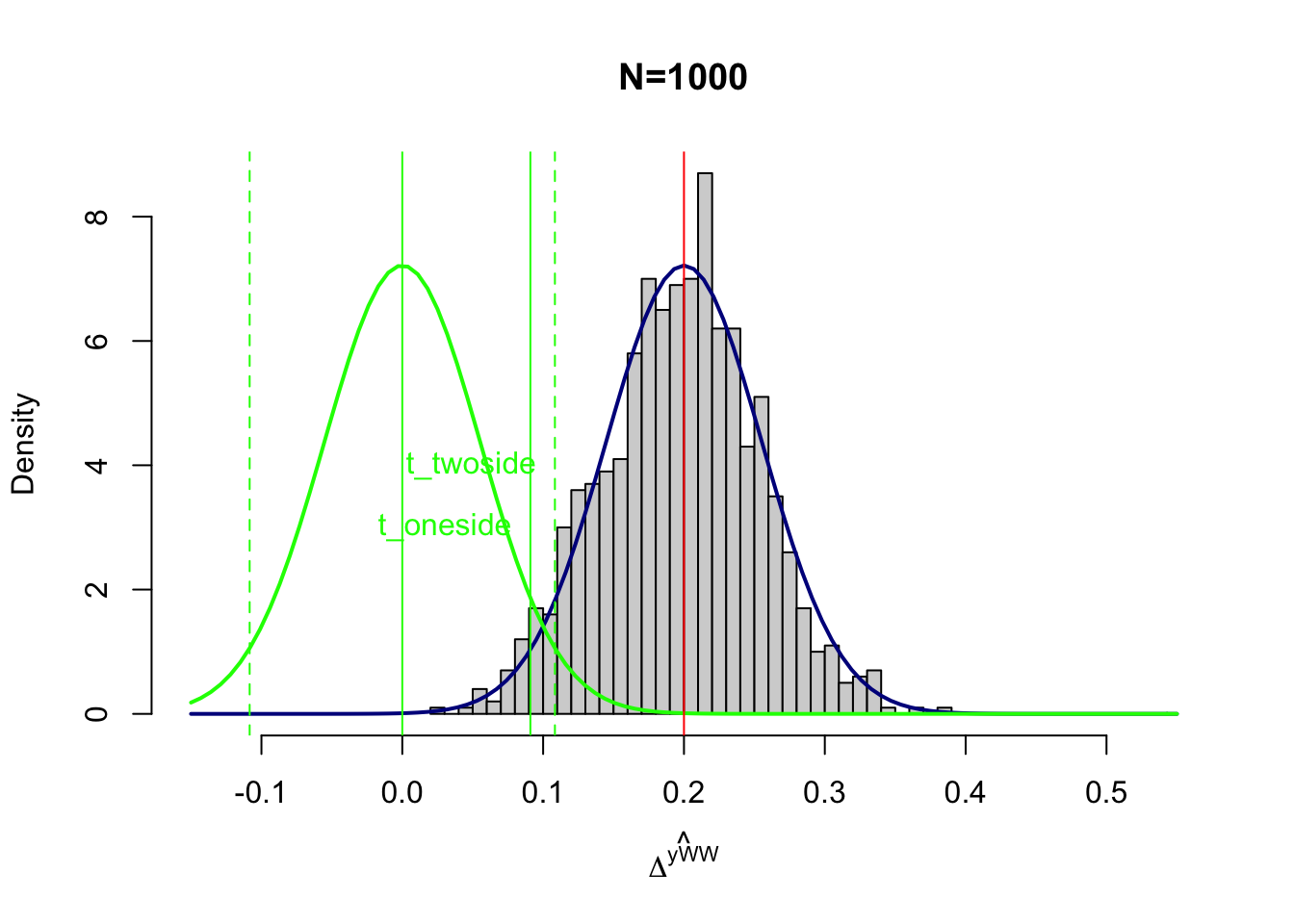
Figure 7.1: Power with \(\beta_A=0.2\)
Figure 7.1 shows the distribution of \(\hat{E}\) under the null in green and the distribution under the alternativein blue. In black is the distribution stemming from the Monte Carlo simulations recentered at \(\beta_A=0.2\). All of these distributions have the same shape (they are normal with variance 0.003) and differ only by their mean.
Under the null of no effect, \(\hat{E}\) would be distributed as the green curve, centered at \(0\). The green continuous vertical line materializes the threshold \(t_{\text{oneside}}=\Phi^{-1}\left(1-\alpha\right)\sqrt{\var{\hat{E}}}\) of the one-sided test (as defined in the proof of Theorem 7.1). The green discontinuous vertical lines materialize the thresholds \(t_{\text{twoside}}=\pm\Phi^{-1}\left(1-\frac{\alpha}{2}\right)\sqrt{\var{\hat{E}}}\) of the two-sided test (as defined in the proof of Theorem 7.1).
We are more accustomed to seeing these thresholds standardized by \(\sqrt{\var{\hat{E}}}\). I find it simpler to visualize their nonstandardized versions. It enables to position the test statistics on the actual distribution of \(\hat{E}\) and to compare their values with the values of the parameter estimates. Note that you can easily go back between the classical standardized thresholds for the test statistics and the nonstandardized ones by dividing and multiplying by \(\sqrt{\var{\hat{E}}}\). As a result, we find that the standardized threshold for the one sided test, \(\frac{t_{\text{oneside}}}{\sqrt{\var{\hat{E}}}}=\Phi^{-1}\left(1-\alpha\right)\), is equal to 1.64, for \(\alpha=\) 0.05. For the two-sided test, the absolute value of the standardized threshold is equal to \(\left|\frac{t_{\text{twoside}}}{\sqrt{\var{\hat{E}}}}\right|=\Phi^{-1}\left(1-\frac{\alpha}{2}\right)\), which is equal to 1.96, for \(\alpha=\) 0.05. You probably already know these threshold values, especially the second one, as the classical threshold for 5% statistical significance in t-tests for the null of an estimated parameter being zero.
What we are doing here is express the thresholds of the test statistics as multiples of the standard error of the estimated parameter.
For a one-sided test, we consider as statistically significant an estimated effect that is 1.64 times larger than its standard error, and for a two-sided test, an estimated effect whose larger in absolute value than 1.96 its standard error.
Because the distribution of \(\hat{E}\) is normal, under Assumption 7.1, the probability that the value of \(\hat{E}\) falls above these thresholds under the null is equal to \(\alpha=\) 0.05.
More precisely, for the one sided test, the probability that \(\hat{E}\) falls above \(t_{\text{oneside}}\) under the null is 5%.
For the two-sided test, it is the probability that \(\hat{E}\) falls above \(t_{\text{twoside}}\) or below \(-t_{\text{twoside}}\) under the null that is equal to 5%.
Or, stated otherwise, it is the probability that \(|\hat{E}|>t_{\text{twoside}}\) which is equal to 5% under the null for the two-sided test.
In practice, with our current choice of parameter values (especially the variance of \(\hat{E}\)), we have \(t_{\text{oneside}}=\) 0.09 and \(t_{\text{twoside}}=\) 0.11.
If the estimated treatment effect falls above these threshold values, a one-sided and a two-sided test respectively will find that these effects are statistically significantly different from zero at 5%.
Power computation does not stop there. It asks the following question: if the true value of \(E\) is actually \(E=\beta_A\), what is the probability that our estimator \(\hat{E}\) will fall above \(t_{\text{oneside}}\) or \(t_{\text{twoside}}\)?
Before going further, note that if \(\beta_A>0\) and \(\var{\hat{E}}\) is not too large, the probability that \(\hat{E}\) falls below \(-t_{\text{twoside}}\) under the alternative hypothesis is negligible. It is materialized on Figure 7.1 as the area under the the portion of the blue curve below the lower discontinuous vertical green line positioned at \(-t_{\text{twoside}}=\) -0.11. It is obviously very small. We know from Assumption 7.1 that this probability is equal to \(\Pr(\hat{E}\leq -t_{\text{twoside}})=\Phi\left(\frac{-t_{\text{twoside}}-\beta_A}{\sqrt{\var{\hat{E}}}}\right)=\) 1.2224593^{-8}.
So now, what is the probability that \(\hat{E}\) falls above \(t_{\text{oneside}}\) or \(t_{\text{twoside}}\) under the assumption that \(E=\beta_A>0\)? Intuitively, it is the area under the portion of the blue curve which is above the continuous green vertical line positioned at \(t_{\text{oneside}}=\) 0.09 or above the discontinuous green vertical line positioned at \(t_{\text{twoside}}=\) 0.11. Because we know that \(\hat{E}\) follows a normal with mean \(\beta_A\) and variance \(\var{\hat{E}}\) under the alternative, we can compute these quantities as equal to \(\kappa_{t}=1-\Phi\left(\frac{t-\beta_A}{\sqrt{\var{\hat{E}}}}\right)=\Phi\left(\frac{\beta_A-t}{\sqrt{\var{\hat{E}}}}\right)\), for \(t\in\left\{\text{oneside},\text{twoside}\right\}\). Note that using the formulae for \(t_{\text{oneside}}\) and \(t_{\text{twoside}}\) yields the results in Theorem 7.1. In practice, we have \(\kappa_{\text{oneside}}=\) 0.98 and \(\kappa_{\text{twoside}}=\) 0.95.
What would happen to power if \(\beta_A\) was lower? For example, what if \(\beta_A=0.1\)?
betaA <- 0.1
hist(simuls.brute.force.ww[['1000']][,'WW']-delta.y.ate(param)+betaA,breaks=30,main='N=1000',xlab=expression(hat(Delta^yWW)),xlim=c(-0.15,0.55),probability=T)
curve(dnorm(x, mean=betaA, sd=sqrt(varE)),col="darkblue", lwd=2, add=TRUE, yaxt="n")
curve(dnorm(x, mean=0, sd=sqrt(varE)),col="green", lwd=2, add=TRUE, yaxt="n")
abline(v=betaA,col="red")
abline(v=qnorm(1-alpha)*sqrt(varE),col="green")
abline(v=qnorm(1-alpha/2)*sqrt(varE),col="green",lty=lty.unobs)
abline(v=-qnorm(1-alpha/2)*sqrt(varE),col="green",lty=lty.unobs)
abline(v=0,col="green")
text(x=c(qnorm(1-alpha)*sqrt(varE),qnorm(1-alpha/2)*sqrt(varE)),y=c(adj+3,adj+4),labels=c('t_oneside','t_twoside'),pos=c(2,2),col=c('green','green'),lty=c(lty.obs,lty.unobs))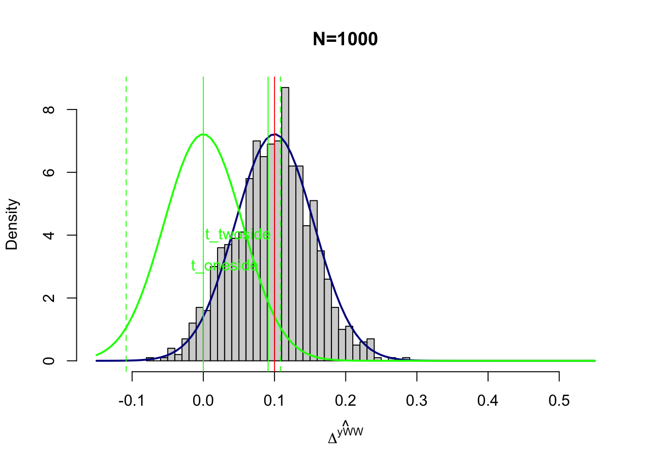
Figure 7.2: Power with \(\beta_A=0.1\)
Figure 7.2 shows what would happen with \(\beta_A=0.1\). It becomes much harder to tell the green curve from the blue curve. As a consequence, power decreases, since the portion of the blue curve located below the thresholds increases. It is a consequence less likely that a t-test will reject the assumption that the treatment effect is zero, even when it is not zero but equal to \(0.1\). How less likely? Well, power is now equal to \(\kappa_{\text{oneside}}=\) 0.57 and \(\kappa_{\text{twoside}}=\) 0.44.
What would happen now if our estimator was way more precise? For example, what would happen if we could reach the precision of the With/Without estimator with a sample size of \(N=10000\) instead of \(N=1000\) as we have assumed up to now?
betaA <- 0.2
varE.10000 <- var(simuls.brute.force.ww[['10000']][,'WW'])

hist(simuls.brute.force.ww[['10000']][,'WW']-delta.y.ate(param)+betaA,breaks=30,main='N=10000',xlab=expression(hat(Delta^yWW)),xlim=c(-0.15,0.55),probability=T)
curve(dnorm(x, mean=betaA, sd=sqrt(varE)),col="darkblue", lwd=2, add=TRUE, yaxt="n")
curve(dnorm(x, mean=betaA, sd=sqrt(varE.10000)),col="darkblue", lwd=2, add=TRUE, yaxt="n")
curve(dnorm(x, mean=0, sd=sqrt(varE)),col="green", lwd=2, add=TRUE, yaxt="n")
curve(dnorm(x, mean=0, sd=sqrt(varE.10000)),col="green", lwd=2, add=TRUE, yaxt="n")
abline(v=betaA,col="red")
abline(v=qnorm(1-alpha)*sqrt(varE),col="green")
abline(v=qnorm(1-alpha/2)*sqrt(varE),col="green",lty=lty.unobs)
abline(v=-qnorm(1-alpha/2)*sqrt(varE),col="green",lty=lty.unobs)
abline(v=qnorm(1-alpha)*sqrt(varE.10000),col="green")
abline(v=qnorm(1-alpha/2)*sqrt(varE.10000),col="green",lty=lty.unobs)
abline(v=-qnorm(1-alpha/2)*sqrt(varE.10000),col="green",lty=lty.unobs)
abline(v=0,col="green")
text(x=c(qnorm(1-alpha)*sqrt(varE),qnorm(1-alpha/2)*sqrt(varE)),y=c(adj+3,adj+4),labels=c('t_oneside','t_twoside'),pos=c(2,2),col=c('green','green'),lty=c(lty.obs,lty.unobs))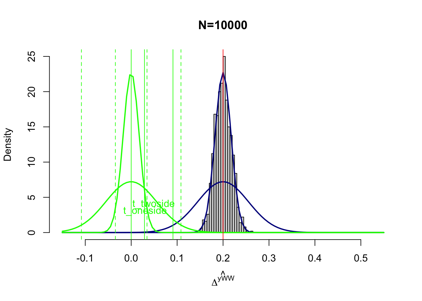
Figure 7.3: Power with \(N=10000\)
Figure 7.3 shows what would happen with \(\beta_A=0.2\) and \(N=10000\).
There are two effects of increased precision on power.
First, the blue curve is thinner, which means that less of its area lies before the thresholds of the test statisics.
Second, the green curve is also thinner, which means that the threshold are smaller.
With \(N=10000\), \(t_{\text{oneside}}=\) 0.029 and \(t_{\text{twoside}}=\) 0.034.
As a consequence, power increases sharply with \(N=10000\).
For \(\beta_A=0.2\), power is now \(\kappa_{\text{oneside}}=\) 1 and \(\kappa_{\text{twoside}}=\) 1.
For \(\beta_A=0.1\), power is now \(\kappa_{\text{oneside}}=\) 1 and \(\kappa_{\text{twoside}}=\) 1.
Finally, let us see how power changes with \(\var{\hat{E}}\) (through sample size), \(\beta_A\) and \(\alpha\). Let us first run some simulations:
varE.N <- c(var(simuls.brute.force.ww[['100']][,'WW']),var(simuls.brute.force.ww[['1000']][,'WW']),var(simuls.brute.force.ww[['10000']][,'WW']),var(simuls.brute.force.ww[[4]][,'WW']))

alpha <- 0.05
betaA <- 0.2
power.N.05.02 <- sapply(varE.N,power,alpha=alpha,betaA=betaA)
power.N.twoside.05.02 <- sapply(varE.N,power.twoside,alpha=alpha,betaA=betaA)

betaA <- 0.1
power.N.05.01 <- sapply(varE.N,power,alpha=alpha,betaA=betaA)
power.N.twoside.05.01 <- sapply(varE.N,power.twoside,alpha=alpha,betaA=betaA)

alpha <- 0.01
power.N.01.01 <- sapply(varE.N,power,alpha=alpha,betaA=betaA)
power.N.twoside.01.01 <- sapply(varE.N,power.twoside,alpha=alpha,betaA=betaA)

betaA <- 0.2
power.N.01.02 <- sapply(varE.N,power,alpha=alpha,betaA=betaA)
power.N.twoside.01.02 <- sapply(varE.N,power.twoside,alpha=alpha,betaA=betaA)

N.sample <- c(100,1000,10000,100000)
power.sample <- data.frame("N"=rep(N.sample,8),"Power"=c(power.N.05.02,power.N.twoside.05.02,power.N.05.01,power.N.twoside.05.01,power.N.01.01,power.N.twoside.01.01,power.N.01.02,power.N.twoside.01.02))
colnames(power.sample) <- c('N','Power')
power.sample$Test <- rep(c(rep('One-sided',length(N.sample)),rep('Two-sided',length(N.sample))),4)
power.sample$betaA <- c(rep(0.2,2*length(N.sample)),rep(0.1,4*length(N.sample)),rep(0.2,2*length(N.sample)))
power.sample$alpha <- c(rep(0.05,4*length(N.sample)),rep(0.01,4*length(N.sample)))
Let us now plot the resulting estimates:
ggplot(power.sample, aes(x=as.factor(N), y=Power, fill=Test)) +
  geom_bar(position=position_dodge(), stat="identity") +
  xlab("Sample Size") +
  theme_bw()+
  facet_grid(betaA~alpha)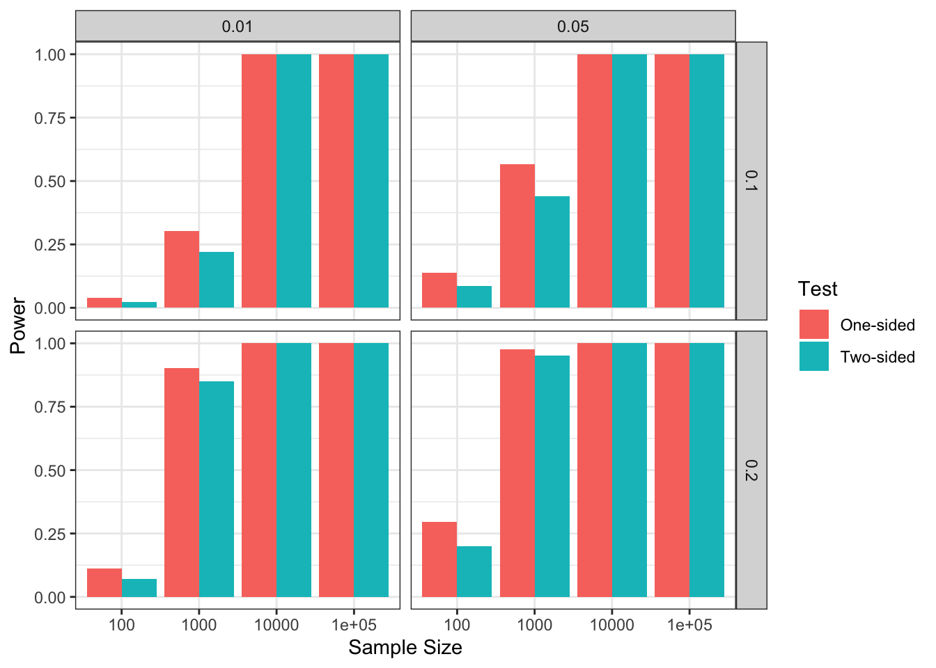
Figure 7.4: Power and Sample Size as a function of \(\alpha\) (left vs right) and \(\beta_A\) (top vs bottom)
Figure 7.4 shows that sample size is a key determinant of power, but that \(\alpha\) and \(\beta_A\) are as well. For example, with \(\beta_A=0.1\) and \(\alpha=0.01\), \(N=1000\) has low power (around \(0.25\)). Moving to sample size \(N=10000\) would ensure very effective power, but let us keep \(N=1000\) for now. We can see that simply increasing \(\alpha\) to \(0.05\) increases power to around \(0.5\). But it is increasing \(\beta_A\) to \(0.2\) that has the strongest effect: power is now around \(0.9\), whatever \(\alpha\). As a consequence, choosing \(\beta_A\) correctly is key to ensure a correct power analysis.
7.1.2 Minimum Detectable Effect
In general power analysis does not stop after computing power. We also might want to compute the Minimum Detectable Effect (or MDE) that we can detect with a sample of size \(N\) and a (one- or two-sided) test of size \(\alpha\) with power \(\kappa\). The following theorem enables us to do just that:
Theorem 7.2 (Minimum Detectable Effect with an Asymptotically Normal Estimator) With \(\hat{E}\) complying with Assumption 7.1, the Minimum Detectable Effect of a one- or two-sided test is:
- For a One-Sided Test: \(H_0\): \(E\leq0\) \(H_A\): \(E=\beta_A>0\)
\[\begin{align*} \beta_A^{\text{oneside}} & = \left(\Phi^{-1}\left(\kappa\right)+\Phi^{-1}\left(1-\alpha\right)\right)\sqrt{\var{\hat{E}}}, \end{align*}\]
- For a Two-Sided Test: \(H_0\): \(E=0\) \(H_A\): \(E=\beta_A\neq0\)
\[\begin{align*} \beta_A^{\text{twoside}} & \approx \left(\Phi^{-1}\left(\kappa\right)+\Phi^{-1}\left(1-\frac{\alpha}{2}\right)\right)\sqrt{\var{\hat{E}}}. \end{align*}\]
Proof. Using Theorem 7.1, inverting the power formula yields the result.
With Theorem 7.2, we have a way to compute the MDE for a wide range of applications, as long as we know \(\var{\hat{E}}\) and that we have choosen properly \(\alpha\) and \(\kappa\). In most applications, researchers choose \(\alpha=0.05\) and \(\kappa=0.8\), so that they compute the effect that they have 80% chance to detect with a test of size 5%.
Example 7.2 In our example, we can try to see what the MDE looks for various sample sizes. Let us first write functions to compute the MDE:
MDE.var <- function(alpha,kappa,varE,oneside){
  if (oneside==TRUE){
    MDE <- (qnorm(kappa)+qnorm(1-alpha))*sqrt(varE)
  }
  if (oneside==FALSE){
    MDE <- (qnorm(kappa)+qnorm(1-alpha/2))*sqrt(varE)
  }
  return(MDE)
}
MDE <- function(N,alpha,kappa,CE,oneside){
  if (oneside==TRUE){
    MDE <- (qnorm(kappa)+qnorm(1-alpha))*sqrt(CE/N)
  }
  if (oneside==FALSE){
    MDE <- (qnorm(kappa)+qnorm(1-alpha/2))*sqrt(CE/N)
  }
  return(MDE)
}

alpha <- 0.05
kappa <- 0.8
MDE.N.oneside <- sapply(varE.N,MDE.var,alpha=alpha,kappa=kappa,oneside=TRUE)
MDE.N.twoside <- sapply(varE.N,MDE.var,alpha=alpha,kappa=kappa,oneside=FALSE)
power.sample$MDE <- c(MDE.N.oneside,MDE.N.twoside)
Let us now plot the results:
ggplot(power.sample, aes(x=as.factor(N), y=MDE,fill=Test)) +
  geom_bar(position=position_dodge(), stat="identity") +
  xlab("Sample Size") +
  theme_bw()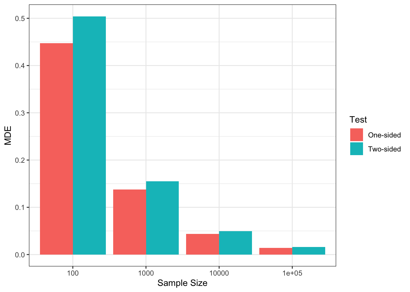
Figure 7.5: MDE and Sample Size
Figure 7.5 shows that, with \(\alpha=\) 0.05 and \(\kappa=\) 0.8 and a two-sided test, we can detect a minimum effect of 0.5 with \(N=\) 100, whereas the MDE decreases to 0.15 with \(N=\) 1000 and even further to 0.05 with \(N=\) 10^{4} and 0.02 with \(N=\) 10^{5}.
7.1.3 Minimum Required Sample Size
Finally, we can also estimate the minimum sample size required to estimate an effect with given size and power. The following theorem shows how:
Theorem 7.3 (Minimum Required Sample Size with an Asymptotically Normal Estimator) With \(\hat{E}\) complying with Assumption 7.1, the Minimum Required Sample Size to estimate an effect \(\beta_A\) with a one- or two-sided test is:
- For a One-Sided Test: \(H_0\): \(E\leq0\) \(H_A\): \(E=\beta_A>0\)
\[\begin{align*} N_{\text{oneside}} & = \left(\Phi^{-1}\left(\kappa\right)+\Phi^{-1}\left(1-\alpha\right)\right)^2\frac{C(\hat{E})}{\beta_A^2}, \end{align*}\]
- For a Two-Sided Test: \(H_0\): \(E=0\) \(H_A\): \(E=\beta_A\neq0\)
\[\begin{align*} N_{\text{twoside}} & = \left(\Phi^{-1}\left(\kappa\right)+\Phi^{-1}\left(1-\frac{\alpha}{2}\right)\right)^2\frac{C(\hat{E})}{\beta_A^2}. \end{align*}\]
Proof. Using Theorem 7.2, and inverting the formula for MDE yields the result.
Example 7.3 Let us see how this works in our example. Let us first write a function to compute the required formulae and then set up \(C(\hat{E})\) and finally the minimum reauired sample size for a given treatment effect:
# formula
sample.size <- function(betaA,alpha,kappa,CE,oneside){
  if (oneside==TRUE){
    N <- (qnorm(kappa)+qnorm(1-alpha))^2*(CE/(betaA^2))
  }
  if (oneside==FALSE){
    N <- (qnorm(kappa)+qnorm(1-alpha/2))^2*(CE/(betaA^2))
  }
  return(round(N))
}
# C(E)
C.E.N <- varE.N*N.sample
# choose set of MDEs
MDE.set <- c(1,0.5,0.2,0.1,0.02)
# compute set of MDEs for a given C(E) (let's choose the one for 1000)
N.mini.oneside <- sapply(MDE.set,sample.size,alpha=alpha,kappa=kappa,CE=C.E.N[[2]],oneside=TRUE)
N.mini.twoside <- sapply(MDE.set,sample.size,alpha=alpha,kappa=kappa,CE=C.E.N[[2]],oneside=FALSE)
# Data frame
MDE.N.sample <- data.frame("betaA"=rep(MDE.set,2),"N"=c(N.mini.oneside,N.mini.twoside),"Test"=rep(c(rep('One-sided',length(MDE.set)),rep('Two-sided',length(MDE.set)))))
Let us now plot the results:
ggplot(MDE.N.sample, aes(x=as.factor(betaA), y=N,fill=Test)) +
  geom_bar(position=position_dodge(), stat="identity") +
  xlab("betaA") +
  ylab("Sample size (log scale)")+
  yscale("log10",.format=TRUE)+
  theme_bw()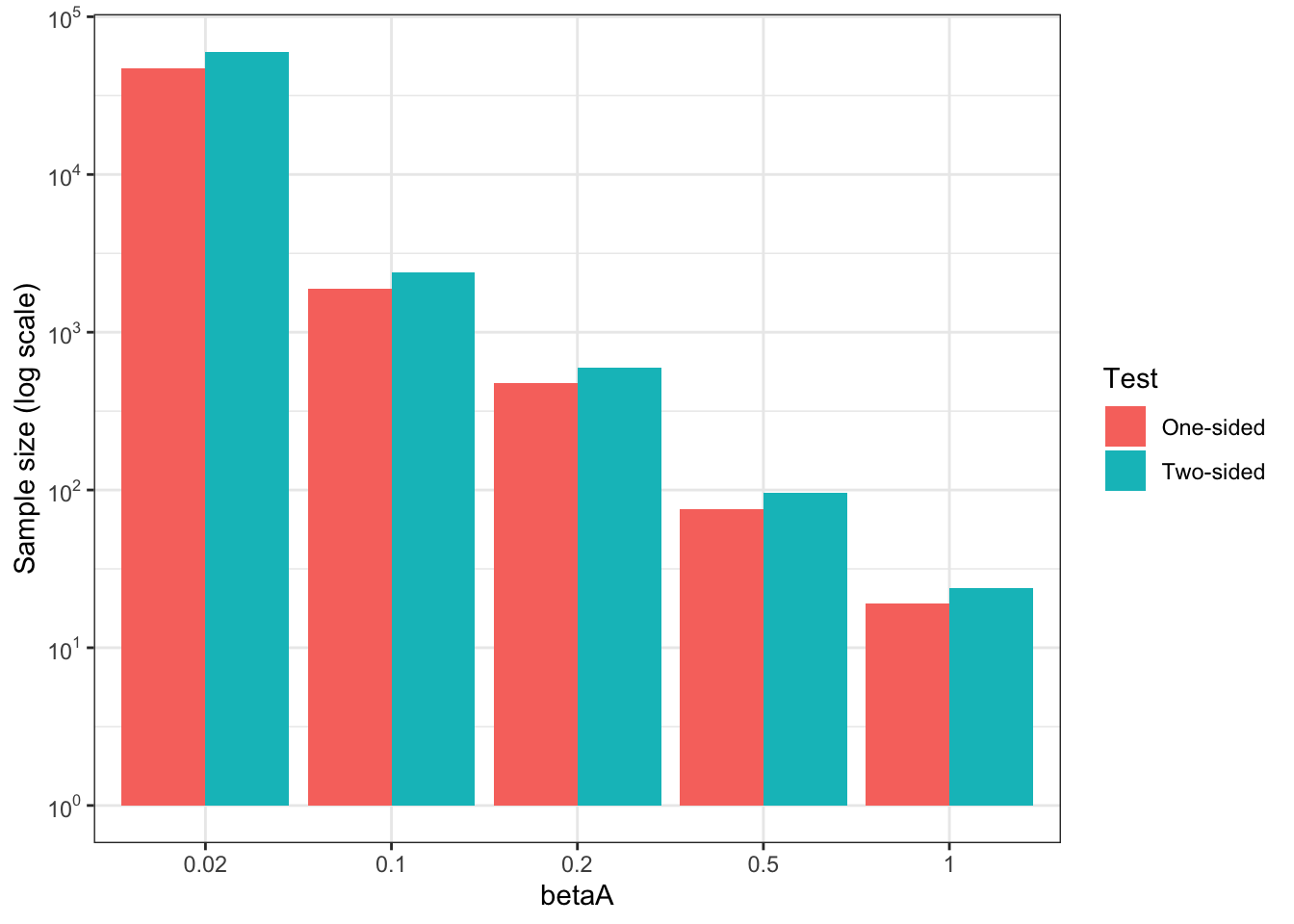
Figure 7.6: Minimum required sample size
Figure 7.6 shows that Minimum Required Sample Size increases very fast as \(\beta_A\), the minimum effect to detect, decreases. For \(\beta_A=\) 1, the Minimum Required Sample Size is equal to 24. For \(\beta_A=\) 0.5, the Minimum Required Sample Size is equal to 96. For \(\beta_A=\) 0.2, the Minimum Required Sample Size is equal to 600. For \(\beta_A=\) 0.1, the Minimum Required Sample Size is equal to 2400. For \(\beta_A=\) 0.02, the Minimum Required Sample Size is equal to 5.9988^{4}.
7.2 Traditional power analysis in practice
In the previous section, we have covered the basics of power analysis. In order to implement it in practice, we still need an estimate of \(\var{\hat{E}}\) or of \(C(\hat{E})\). When we want to compute power after we have estimated an effect, both of these quantities can easily be recovered from most estimators we have covered in this book. One problem, though, is when we want to conduct a power analysis before running a study (for example, before collecting the data). There, we need a way to find a reasonable estimate of \(\var{\hat{E}}\) and \(C(\hat{E})\). We are going to see several ways of doing that, but basically, we need prior information on the properties of our outcomes and covariates. They can come from baseline data or from data take in a similar population as our target population. Sometimes, we have to make strong assumptions to move the results from one population to our target population. Let’s examine in practice how to do that, in the context of all the econometric methods we have studied so far.
7.2.1 Power Analysis for Randomized Controlled Trials
We are going to decompose what needs to be done for each of the four RCT designs we have studied in Section 3.
7.2.1.1 Power Analysis for Brute Force Designs
For Brute Force designs, the mosts straightforward way to do a power analysis is to rely on the CLT-based approximation for the precision of our estimator. Using Theorem 2.5 and especially Lemma A.5, we have, in a Brute Force design:
\[\begin{align*} \var{\hat{\Delta}^Y_{WW^{BF}}} & \approx \frac{1}{N}\left(\frac{\var{Y_i^1|R_i=1}}{\Pr(R_i=1)}+\frac{\var{Y_i^0|R_i=0}}{1-\Pr(R_i=1)}\right). \end{align*}\]
We can see that Assumption 7.1 is valid for this estimator.
In order to compute \(\var{\hat{\Delta}^Y_{WW}}\) of \(C(\hat{\Delta}^Y_{WW})\), we need to come up with reasonable estimates of \(\var{Y_i^1|R_i=1}\) and \(\var{Y_i^0|R_i=0}\). The problem is that these quantities will only be revealed after the treatment has been given. It is fine for ex-post power analysis but is not feasible for ex-ante power analysis.
One way around this issue is to use an estimate of the variance of \(Y_i\) in a related or similar sample to benchmark our formula. In our case, we can use the variance of \(Y_i^B\), outcomes observed in the period before the treatment is taken, as a source of estimates. Since we cannot know who will get the treatment and who will not, we are going to use the same benchmark for both (\(\var{Y_i^B}\)). This is not perfect but this is what we have. As a result, our estimate of \(C(\hat{\Delta}^Y_{WW})\) in the brute force design is:
\[\begin{align*} \hat{C}(\hat{\Delta}^Y_{WW^{BF}}) & = \frac{\var{Y_i^B}}{p(1-p)}, \end{align*}\]
where \(p\) is the proportion of individuals in our sample who will be allocated to the treatment.
Example 7.4 Let us see how this formula works out in our example. First, we need to generate a sample:
set.seed(1234)
N <-1000
mu <- rnorm(N,param["barmu"],sqrt(param["sigma2mu"]))
UB <- rnorm(N,0,sqrt(param["sigma2U"]))
yB <- mu + UB
YB <- exp(yB)
Ds <- rep(0,N)
Ds[YB<=param["barY"]] <- 1
epsilon <- rnorm(N,0,sqrt(param["sigma2epsilon"]))
eta<- rnorm(N,0,sqrt(param["sigma2eta"]))
U0 <- param["rho"]*UB + epsilon
y0 <- mu +  U0 + param["delta"]
alpha.i <- param["baralpha"]+  param["theta"]*mu + eta
y1 <- y0+alpha.i
Y0 <- exp(y0)
Y1 <- exp(y1)
# randomized allocation of 50% of individuals
Rs <- runif(N)
R <- ifelse(Rs<=.5,1,0)
y <- y1*R+y0*(1-R)
Y <- Y1*R+Y0*(1-R)
Let us now compute the minimum detectable effect for various sample sizes and proportions of treated individuals, using \(\hatvar{y^B_i}=\) 0.78 as an estimate of \(\hatvar{y_i^1|R_i=1}=\) 0.85 and \(\hatvar{y_i^0|R_i=0}=\) 0.78.
CE.BF.fun <- function(p,varYb){
  return(varYb/(p*(1-p)))
}

MDE.BF.fun <- function(p,varYb,...){
  return(MDE(CE=CE.BF.fun(p=p,varYb=varYb),...))
}
Let us finally check what Minimum Detectable Effect looks like as a function of \(p\) and of sample size.
ggplot() +
  xlim(0,1) +
  ylim(0,1) +
  geom_function(aes(color="100"),fun=MDE.BF.fun,args=list(N=100,varYb=var(yB),alpha=alpha,kappa=kappa,oneside=FALSE)) +
  geom_function(aes(color="1000"),fun=MDE.BF.fun,args=list(N=1000,varYb=var(yB),alpha=alpha,kappa=kappa,oneside=FALSE)) +
  geom_function(aes(color="10000"),fun=MDE.BF.fun,args=list(N=10000,varYb=var(yB),alpha=alpha,kappa=kappa,oneside=FALSE)) +
  geom_function(aes(color="100000"),fun=MDE.BF.fun,args=list(N=100000,varYb=var(yB),alpha=alpha,kappa=kappa,oneside=FALSE)) +
  scale_color_discrete(name="N") +
  ylab("MDE") +
  xlab("p") +
  theme_bw()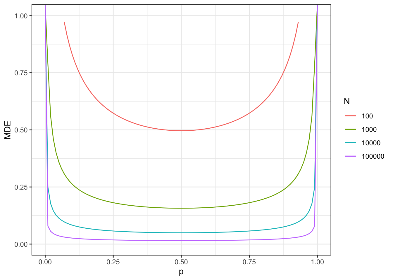
Figure 7.7: Minimum detectable effect for the Brute Force design
As figure 7.7 shows, the Minimum Detectable Effect is minimized, for a given sample size, at \(p=0.5\). This makes sense since it is where we get the most precision out of our treated and control samples. This results depends crucially on the fact that we have assumed no heteroskedasticity (i.e. that we have assumed that the variance of outcomes does not change with treatment status). We also can see that MDE decreases with sample size, but slower than proportionally. Again, it makes sense, since power and MDE depend on the square root of sample size.
With a sample size of \(N=100\), we now reach a MDE of 0.5.
With a sample size of \(N=1000\), we now reach a MDE of 0.16.
With a sample size of \(N=10000\), we now reach a MDE of 0.05.
With a sample size of \(N=100000\), we now reach a MDE of 0.02.
7.2.1.2 Power Analysis for Self-Selection Designs
For self-selection designs, the approach is similar to that of brute force designs, except that, since randomization occurs after self-selection, you have to make a guess on the proportion of people who will take the treatment. We have:
\[\begin{align*} \var{\hat{\Delta}^Y_{WW^{SS}}} & \approx \frac{1}{N}\frac{1}{\Pr(D_i=1)}\left(\frac{\var{Y_i^1|D_i=1,R_i=1}}{\Pr(R_i=1|D_i=1)}+\frac{\var{Y_i^0|D_i=1,R_i=0}}{1-\Pr(R_i=1|D_i=1)}\right), \end{align*}\]
with \(N\) the total number of individuals in the sample, including the inegilible individuals and the individuals who do not self-select into the program. Estimates of the MDE and of the Minimum Required Sample Size can be expressed in terms of \(N\) or of \(N^D=N\Pr(D_i=1)\), the number of individuals who self-select into the program and among which randomization is run.
The estimates we need to compute these quantities are more complex than with brute force designs: we need \(\Pr(D_i=1)\), but also variances conditional on \(D_i=1\). If the program was operating before randomization, we can have some pretty good ideas of these numbers. Otherwise, we have to use either surveys on intentions to participate, or evidence from similar programs, or at least try to enforce the eligibility criteria as much as we can.
Example 7.5 Let’s see how we can make this work in our example.
Let us first update our parameters for modelling self-selection, as we did in Chapter 3:
param <- c(param,-6.25,0.9,0.5)
names(param) <- c("barmu","sigma2mu","sigma2U","barY","rho","theta","sigma2epsilon","sigma2eta","delta","baralpha","barc","gamma","sigma2V")
and let’s generate a new dataset:
set.seed(1234)
N <-1000
mu <- rnorm(N,param["barmu"],sqrt(param["sigma2mu"]))
UB <- rnorm(N,0,sqrt(param["sigma2U"]))
yB <- mu + UB
YB <- exp(yB)
E <- ifelse(YB<=param["barY"],1,0)
V <- rnorm(N,0,param["sigma2V"])
Dstar <- param["baralpha"]+param["theta"]*param["barmu"]-param["barc"]-param["gamma"]*mu-V
Ds <- ifelse(Dstar>=0 & E==1,1,0)
epsilon <- rnorm(N,0,sqrt(param["sigma2epsilon"]))
eta<- rnorm(N,0,sqrt(param["sigma2eta"]))
U0 <- param["rho"]*UB + epsilon
y0 <- mu +  U0 + param["delta"]
alpha <- param["baralpha"]+  param["theta"]*mu + eta
y1 <- y0+alpha
Y0 <- exp(y0)
Y1 <- exp(y1)
#random allocation among self-selected
Rs <- runif(N)
R <- ifelse(Rs<=.5 & Ds==1,1,0)
y <- y1*R+y0*(1-R)
Y <- Y1*R+Y0*(1-R)

# computing application rate
pDhat <- mean(Ds)
We are going to assume that all conditional variances are equal to the pre-treatment variance: we use \(\hatvar{y^B_i}=\) 0.78 as an estimate of \(\hatvar{y_i^1|D_i=1,R_i=1}=\) 0.3 and \(\hatvar{y_i^0|D_i=1,R_i=0}=\) 0.23. This is obviously not a great choice since people with \(D_i=1\) have lower variance in outcomes than the overall population. What happens if we choose instead \(\hatvar{y^B_i|y^B_i\leq\bar{y}}\). Well, \(\hatvar{y^B_i|y^B_i\leq\bar{y}}=\) 0.18, which is a much better guess. So trying to approximate the selection process (at least enforcing the eligibility criteria) is a good idea when doing a power analysis for self-selection designs.
We are going to use:
\[\begin{align*} \hat{C}(\hat{\Delta}^Y_{WW^{SS}}) & = \frac{1}{\Pr(D_i=1)}\frac{\hatvar{y^B_i|y^B_i\leq\bar{y}}}{p(1-p)}, \end{align*}\]
with \(p\) the proportion of applicants randomized into the program.
Let’s write a function to compute the MDE in self-selection designs:
CE.SS.fun <- function(p,varYb,pD){
  return(var(yB)/(pD*p*(1-p)))
}

MDE.SS.fun <- function(p,varYb,pD,...){
  return(MDE(CE=CE.SS.fun(p=p,varYb=varYb,pD=pD),...))
}

alpha <- 0.05
kappa <- 0.8
Let us finally check what Minimum Detectable Effect looks like as a function of \(p\) and of sample size.
# total sample size (including ineligibles and non applicants)
ggplot() +
  xlim(0,1) +
  ylim(0,2) +
  geom_function(aes(color="100"),fun=MDE.SS.fun,args=list(N=100,pD=pDhat,varYb=var(yB[E==1]),alpha=alpha,kappa=kappa,oneside=FALSE)) +
  geom_function(aes(color="1000"),fun=MDE.SS.fun,args=list(N=1000,pD=pDhat,varYb=var(yB[E==1]),alpha=alpha,kappa=kappa,oneside=FALSE)) +
  geom_function(aes(color="10000"),fun=MDE.SS.fun,args=list(N=10000,pD=pDhat,varYb=var(yB[E==1]),alpha=alpha,kappa=kappa,oneside=FALSE)) +
  geom_function(aes(color="100000"),fun=MDE.SS.fun,args=list(N=100000,pD=pDhat,varYb=var(yB[E==1]),alpha=alpha,kappa=kappa,oneside=FALSE)) +
  scale_color_discrete(name="N") +
  ylab("MDE") +
  xlab("p") +
  theme_bw()

# Applicants sample size
pDhat <- 1
ggplot() +
  xlim(0,1) +
  ylim(0,2) +
  geom_function(aes(color="100"),fun=MDE.SS.fun,args=list(N=100,pD=pDhat,varYb=var(yB[E==1]),alpha=alpha,kappa=kappa,oneside=FALSE)) +
  geom_function(aes(color="1000"),fun=MDE.SS.fun,args=list(N=1000,pD=pDhat,varYb=var(yB[E==1]),alpha=alpha,kappa=kappa,oneside=FALSE)) +
  geom_function(aes(color="10000"),fun=MDE.SS.fun,args=list(N=10000,pD=pDhat,varYb=var(yB[E==1]),alpha=alpha,kappa=kappa,oneside=FALSE)) +
  geom_function(aes(color="100000"),fun=MDE.SS.fun,args=list(N=100000,pD=pDhat,varYb=var(yB[E==1]),alpha=alpha,kappa=kappa,oneside=FALSE)) +
  scale_color_discrete(name=expression(N^D)) +
  ylab("MDE") +
  xlab("p") +
  theme_bw()

# computing application rate
pDhat <- mean(Ds)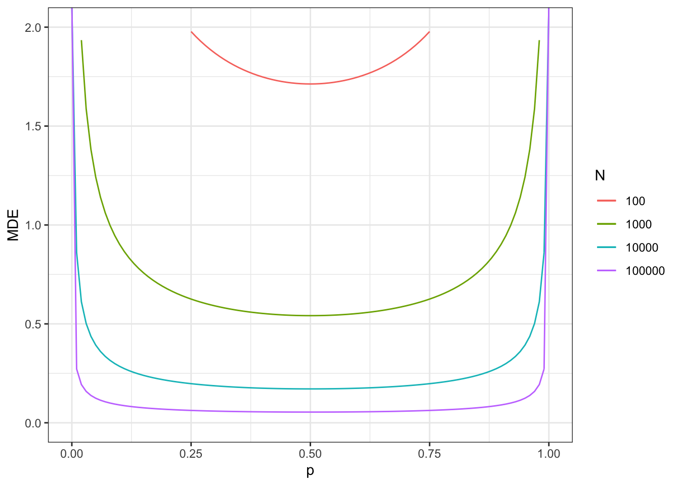
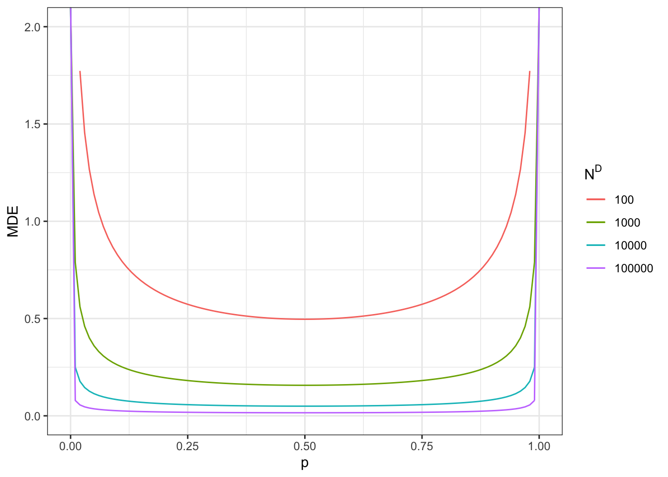
Figure 7.8: Minimum detectable effect for the self-selection design
With a total sample size of \(N=100\), we now reach a MDE of 1.71.
With a total sample size of \(N=1000\), we now reach a MDE of 0.54.
With a total sample size of \(N=10000\), we now reach a MDE of 0.17.
With a total sample size of \(N=100000\), we now reach a MDE of 0.05.
Remember that these sample sizes include ineligible units and units that do not apply for the program. Figure 7.8 also shows what happens when sample size corresponds to only applicants to the program (plot on the right). MDEs in that case look much more like the ones in the brute force design presented in Figure 7.7.
With a total sample size of \(N^D=100\), we now reach a MDE of 0.5.
With a total sample size of \(N^D=1000\), we now reach a MDE of 0.16.
With a total sample size of \(N^D=10000\), we now reach a MDE of 0.05.
With a total sample size of \(N^D=100000\), we now reach a MDE of 0.02.
7.2.1.3 Power Analysis for Eligibility Designs
In eligibility designs, we can make use Theorem 3.8 to show that:
\[\begin{align*} \var{\hat{\Delta}^Y_{Bloom}} & \approx \frac{1}{N}\frac{1}{p^{E}}\frac{1}{(p^{D}_1)^2}\left[\left(\frac{p^D}{p^R}\right)^2\frac{\var{Y_i|R_i=0,E_i=1}}{1-p^R}+\left(\frac{1-p^D}{1-p^R}\right)^2\frac{\var{Y_i|R_i=1,E_i=1}}{p^R}\right], \end{align*}\]
with \(p^E=\Pr(E_i=1)\), \(p^D=\Pr(D_i=1|E_i=1)\), \(p^R=\Pr(R_i=1|E_i=1)\) and \(p^{D}_1=\Pr(D_i=1|R_i=1,E_i=1)\). Note that \(N\) corresponds to the size of the sample including the ineligible individuals which do not enter in the estimation of the treatment effect of the program. MDEs and minimum required sample size can also be expressed in terms of \(N^E=Np^E\), the size of the sample of eligible units.
There is a large number of parameters to find in order to compute this variance estimator. We need to postulate a value for \(p^{E}\) (unless we look for information on the sample size of the eligible population participating in the experiment, in which case we set \(p^{E}=1\) and \(N=N^E\) in the above formula), a value for \(p^D\), for \(p^R\) and for \(p^D_1\). For estimating \(p^E\), we are going to choose the proportion of individuals eligible to the program (\(\hat{p}^E=\Pr(y_i^B\leq\bar{y})\)). For \(p^D\), we know that: \(p^D=\Pr(D_i=1|E_i=1)=\Pr(D_i=1|R_i=1,E_i=1)\Pr(R_i=1|E_i=1)=p^{D}_1p^R\). Since we can vary \(p^R\), we only need to settle on a value for \(p^{D}_1\). We are going to choose the actual value of \(\Pr(D_i=1|R_i=1,E_i=1)\), or \(\hat{p}^{D}_1=\) 1. Finally, we are going to assume that all conditional variances are equal to the pre-treatment variance among eligibles: we use \(\hatvar{y^B_i|E_i=1}=\) 0.18 as an estimate of \(\hatvar{y_i|R_i=1,E_i=1}=\) 0.29 and \(\hatvar{y_i|R_i=0,E_i=1}=\) 0.18.
We can now write \(C(E)\) for the total sample size \(N\) (set \(p^{E}=1\) for \(N=N^E\)):
\[\begin{align*} \hat{C}(\hat{\Delta}^Y_{Bloom}) & = \frac{1}{\hat{p}^{E}}\frac{1}{(\hat{p}^{D}_1)^2}\left[\left(\frac{\hat{p}^D}{p^R}\right)^2\frac{\hatvar{y^B_i|E_i=1}}{1-p^R}+\left(\frac{1-\hat{p}^D}{1-p^R}\right)^2\frac{\hatvar{y^B_i|E_i=1}}{p^R}\right]. \end{align*}\]
Let’s write a function to compute the MDE in eligibility designs:
CE.Elig.fun <- function(pR,varYb,pE,p1D){
  return((1/pE)*(1/p1D)^2*((p1D)^2*varYb/(1-pR)+(((1-p1D*pR)/(1-pR))^2*var(yB)/pR)))
}

MDE.Elig.fun <- function(pR,varYb,pE,p1D,...){
  return(MDE(CE=CE.Elig.fun(pR=pR,varYb=varYb,pE=pE,p1D=p1D),...))
}
# computing candidate participation rate, using the observed proportion below baryB
pEhat <- mean(E)
p1Dhat <- mean(Ds[E==1 & R==1])

alpha <- 0.05
kappa <- 0.8
Let us finally check what Minimum Detectable Effect looks like as a function of \(p^R\) and of sample size.
# total sample size (including ineligibles)
ggplot() +
  xlim(0,1) +
  ylim(0,2) +
  geom_function(aes(color="100"),fun=MDE.Elig.fun,args=list(N=100,pE=pEhat,p1D=p1Dhat,varYb=var(yB[E==1]),alpha=alpha,kappa=kappa,oneside=FALSE)) +
  geom_function(aes(color="1000"),fun=MDE.Elig.fun,args=list(N=1000,pE=pEhat,p1D=p1Dhat,varYb=var(yB[E==1]),alpha=alpha,kappa=kappa,oneside=FALSE)) +
  geom_function(aes(color="10000"),fun=MDE.Elig.fun,args=list(N=10000,pE=pEhat,p1D=p1Dhat,varYb=var(yB[E==1]),alpha=alpha,kappa=kappa,oneside=FALSE)) +
  geom_function(aes(color="100000"),fun=MDE.Elig.fun,args=list(N=100000,pE=pEhat,p1D=p1Dhat,varYb=var(yB[E==1]),alpha=alpha,kappa=kappa,oneside=FALSE)) +
  scale_color_discrete(name="N") +
  ylab("MDE") +
  xlab(expression(p^R)) +
  theme_bw()

# Applicants sample size
pEhat <- 1
ggplot() +
  xlim(0,1) +
  ylim(0,2) +
  geom_function(aes(color="100"),fun=MDE.Elig.fun,args=list(N=100,pE=pEhat,p1D=p1Dhat,varYb=var(yB[E==1]),alpha=alpha,kappa=kappa,oneside=FALSE)) +
  geom_function(aes(color="1000"),fun=MDE.Elig.fun,args=list(N=1000,pE=pEhat,p1D=p1Dhat,varYb=var(yB[E==1]),alpha=alpha,kappa=kappa,oneside=FALSE)) +
  geom_function(aes(color="10000"),fun=MDE.Elig.fun,args=list(N=10000,pE=pEhat,p1D=p1Dhat,varYb=var(yB[E==1]),alpha=alpha,kappa=kappa,oneside=FALSE)) +
  geom_function(aes(color="100000"),fun=MDE.Elig.fun,args=list(N=100000,pE=pEhat,p1D=p1Dhat,varYb=var(yB[E==1]),alpha=alpha,kappa=kappa,oneside=FALSE)) +
  scale_color_discrete(name=expression(N^E)) +
  ylab("MDE") +
  xlab("p") +
  theme_bw()

# computing application rate
pEhat <- mean(E)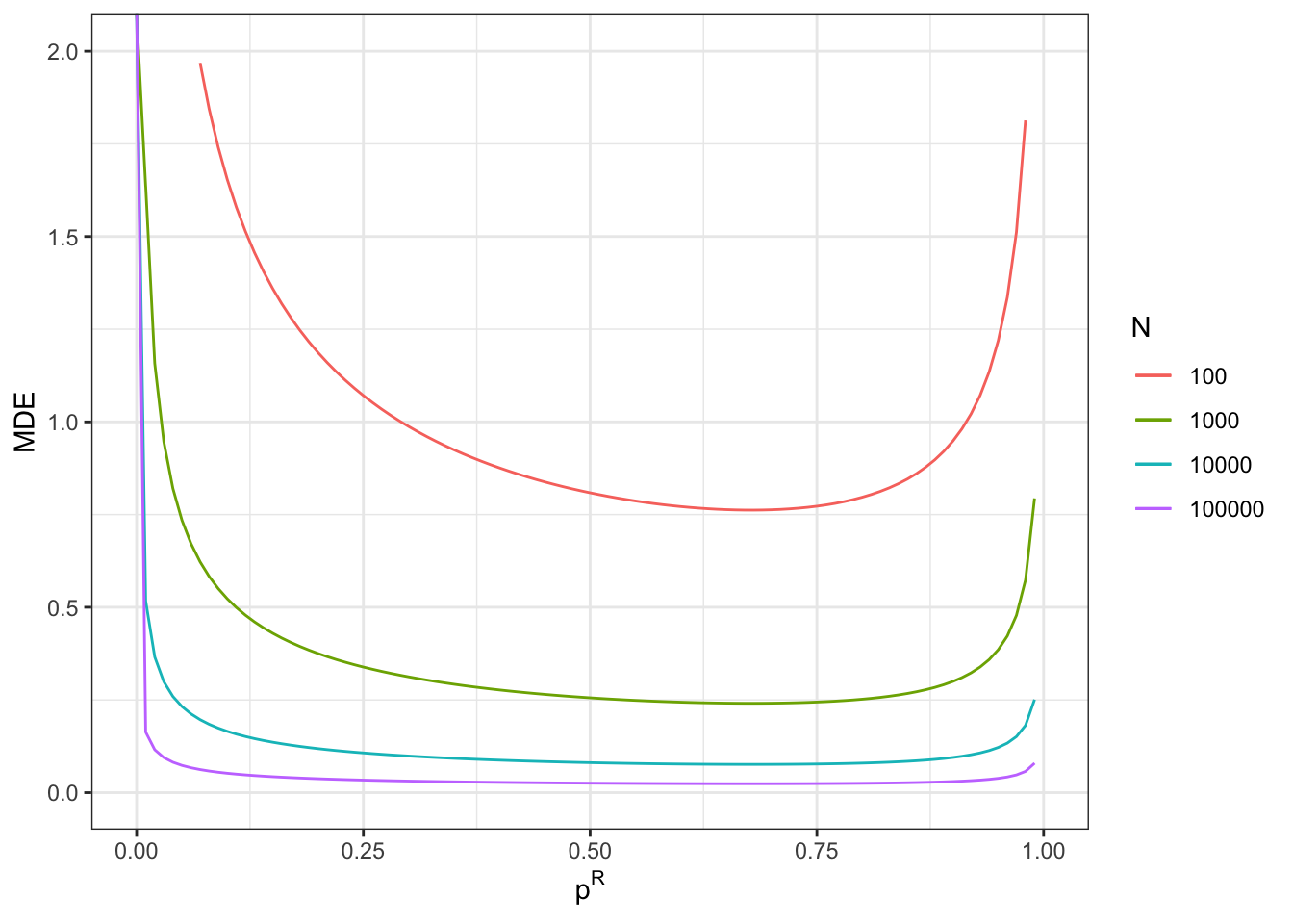
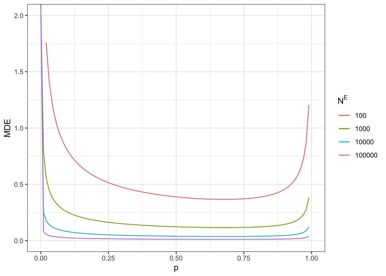
Figure 7.9: Minimum detectable effect for the eligibility design
Note that the minimum detectable effect is no longer minimized at \(p^R=0.5\). We are still going to give the examples at this proportion anyway, since the difference with the optimal proportion of treated is small in our application.
With a total sample size of \(N=100\), we now reach a MDE of 0.81.
With a total sample size of \(N=1000\), we now reach a MDE of 0.26.
With a total sample size of \(N=10000\), we now reach a MDE of 0.08.
With a total sample size of \(N=100000\), we now reach a MDE of 0.03.
Remember that these sample sizes include ineligible units. Figure 7.9 also shows what happens when sample size corresponds to only units eligibles to the program (plot on the right).
With a total sample size of \(N^E=100\), we now reach a MDE of 0.39.
With a total sample size of \(N^E=1000\), we now reach a MDE of 0.12.
With a total sample size of \(N^E=10000\), we now reach a MDE of 0.04.
With a total sample size of \(N^E=100000\), we now reach a MDE of 0.01.
7.2.1.4 Power Analysis for Encouragement Designs
In encouragement designs, we can make use Theorem 3.16 to show that:
\[\begin{align*} \var{\hat{\Delta}^Y_{Wald}} & \approx \frac{1}{N}\frac{1}{p^{E}}\frac{1}{(p^D_1-p^D_0)^2}\left[\left(\frac{p^D}{p^R}\right)^2\frac{\var{Y_i|E_i=1,R_i=0}}{1-p^R}+\left(\frac{1-p^D}{1-p^R}\right)^2\frac{\var{Y_i|E_i=1,R_i=1}}{p^R}\right], \end{align*}\]
with \(p^E=\Pr(E_i=1)\), \(p^D=\Pr(D_i=1|E_i=1)\), \(p^R=\Pr(R_i=1|E_i=1)\), \(p^{D}_0=\Pr(D_i=1|R_i=0,E_i=1)\) and \(p^{D}_1=\Pr(D_i=1|R_i=1,E_i=1)\). Note that \(N\) corresponds to the size of the sample including the ineligible individuals which do not enter in the estimation of the treatment effect of the program. MDEs and minimum required sample size can also be expressed in terms of \(N^E=Np^E\), the size of the sample in terms of eligible units.
As with eligibility designs, there is a large number of parameters to find in order to compute this variance estimator. We need to postulate a value for \(p^{E}\) (unless we look for information on the sample size of the eligible population participating in the experiment, in which case we set \(p^{E}=1\) and \(N=N^E\) in the above formula), a value for \(p^D\), for \(p^R\) and for \(p^D_1\). For estimating \(p^E\), we are going to choose the proportion of individuals eligible to the program (\(\hat{p}^E=\Pr(y_i^B\leq\bar{y})\)). For \(p^D\), we know that: \(p^D=\Pr(D_i=1|E_i=1)=\Pr(D_i=1|R_i=1,E_i=1)\Pr(R_i=1|E_i=1)+\Pr(D_i=1|R_i=0,E_i=1)\Pr(R_i=0|E_i=1)=p^{D}_1p^R+p^{D}_0(1-p^R)\). Since we can vary \(p^R\), we only need to settle on a value for \(p^{D}_1\) and \(p^{D}_0\). We are going to choose their actual values in the sample, \(\Pr(D_i=1|R_i=1,E_i=1)\) and \(\Pr(D_i=1|R_i=0,E_i=1)\), or \(\hat{p}^{D}_1=\) 1 and \(\hat{p}^{D}_0=\) 0.23. In real life applications, this choice is much more difficult. It can for example be based on pilot studies where the response rate to the encouragement is tested. Finally, we are going to assume that all conditional variances are equal to the pre-treatment variance among eligibles: we use \(\hatvar{y^B_i|E_i=1}=\) 0.18 as an estimate of \(\hatvar{y_i|R_i=1,E_i=1}=\) 0.29 and \(\hatvar{y_i|R_i=0,E_i=1}=\) 0.18.
We can now write \(C(E)\) for the total sample size \(N\) (set \(p^{E}=1\) for \(N=N^E\)):
\[\begin{align*} \hat{C}(\hat{\Delta}^Y_{Wald}) & = \frac{1}{\hat{p}^{E}}\frac{1}{(\hat{p}^{D}_1-\hat{p}^{D}_0)^2}\left[\left(\frac{p^{D}_1p^R+p^{D}_0(1-p^R)}{p^R}\right)^2\frac{\hatvar{y^B_i|E_i=1}}{1-p^R}\right.\\ & \phantom{= \frac{1}{\hat{p}^{E}}\frac{1}{(\hat{p}^{D}_1-\hat{p}^{D}_0)^2}\left[\right.}\left.+\left(\frac{1-(p^{D}_1p^R+p^{D}_0(1-p^R))}{1-p^R}\right)^2\frac{\hatvar{y^B_i|E_i=1}}{p^R}\right]. \end{align*}\]
Let’s write a function to compute the MDE in encouragement designs:
CE.Encourage.fun <- function(pR,varYb,pE,p1D,p0D){
  return((1/pE)*(1/(p1D-p0D))^2*(((p1D*pR+p0D*(1-pR))/pR)^2*varYb/(1-pR)+((1-p1D*pR-p0D*(1-pR))/(1-pR))^2*var(yB)/pR))
}

MDE.Encourage.fun <- function(pR,varYb,pE,p1D,p0D,...){
  return(MDE(CE=CE.Encourage.fun(pR=pR,varYb=varYb,pE=pE,p1D=p1D,p0D=p0D),...))
}
# computing candidate participation rate, using the observed proportion below baryB
pEhat <- mean(E)
p1Dhat <- mean(Ds[E==1 & R==1])
p0Dhat <- mean(Ds[E==1 & R==0])

alpha <- 0.05
kappa <- 0.8
Let us finally check what Minimum Detectable Effect looks like as a function of \(p^R\) and of sample size.
# total sample size (including ineligibles)
ggplot() +
  xlim(0,1) +
  ylim(0,2) +
  geom_function(aes(color="100"),fun=MDE.Encourage.fun,args=list(N=100,pE=pEhat,p1D=p1Dhat,p0D=p0Dhat,varYb=var(yB[E==1]),alpha=alpha,kappa=kappa,oneside=FALSE)) +
  geom_function(aes(color="1000"),fun=MDE.Encourage.fun,args=list(N=1000,pE=pEhat,p1D=p1Dhat,p0D=p0Dhat,varYb=var(yB[E==1]),alpha=alpha,kappa=kappa,oneside=FALSE)) +
  geom_function(aes(color="10000"),fun=MDE.Encourage.fun,args=list(N=10000,pE=pEhat,p1D=p1Dhat,p0D=p0Dhat,varYb=var(yB[E==1]),alpha=alpha,kappa=kappa,oneside=FALSE)) +
  geom_function(aes(color="100000"),fun=MDE.Encourage.fun,args=list(N=100000,pE=pEhat,p1D=p1Dhat,p0D=p0Dhat,varYb=var(yB[E==1]),alpha=alpha,kappa=kappa,oneside=FALSE)) +
  scale_color_discrete(name="N") +
  ylab("MDE") +
  xlab(expression(p^R)) +
  theme_bw()

# Applicants sample size
pEhat <- 1
ggplot() +
  xlim(0,1) +
  ylim(0,2) +
  geom_function(aes(color="100"),fun=MDE.Encourage.fun,args=list(N=100,pE=pEhat,p1D=p1Dhat,p0D=p0Dhat,varYb=var(yB[E==1]),alpha=alpha,kappa=kappa,oneside=FALSE)) +
  geom_function(aes(color="1000"),fun=MDE.Encourage.fun,args=list(N=1000,pE=pEhat,p1D=p1Dhat,p0D=p0Dhat,varYb=var(yB[E==1]),alpha=alpha,kappa=kappa,oneside=FALSE)) +
  geom_function(aes(color="10000"),fun=MDE.Encourage.fun,args=list(N=10000,pE=pEhat,p1D=p1Dhat,p0D=p0Dhat,varYb=var(yB[E==1]),alpha=alpha,kappa=kappa,oneside=FALSE)) +
  geom_function(aes(color="100000"),fun=MDE.Encourage.fun,args=list(N=100000,pE=pEhat,p1D=p1Dhat,p0D=p0Dhat,varYb=var(yB[E==1]),alpha=alpha,kappa=kappa,oneside=FALSE)) +
  scale_color_discrete(name=expression(N^E)) +
  ylab("MDE") +
  xlab("p") +
  theme_bw()

# computing application rate
pEhat <- mean(E)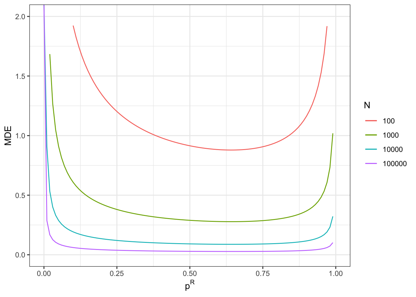
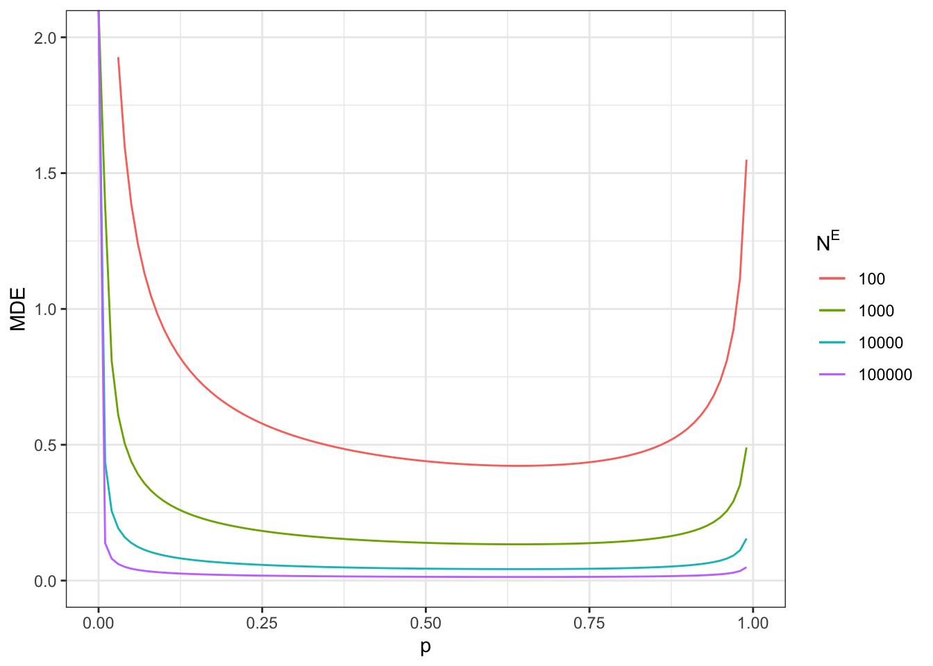
Figure 7.10: Minimum detectable effect for the encouragement design
Note that the minimum detectable effect is no longer minimized at \(p^R=0.5\). We are still going to give the examples at this proportion anyway, since the difference with the optimal proportion of treated is small in our application.
With a total sample size of \(N=100\), we now reach a MDE of 0.91.
With a total sample size of \(N=1000\), we now reach a MDE of 0.29.
With a total sample size of \(N=10000\), we now reach a MDE of 0.09.
With a total sample size of \(N=100000\), we now reach a MDE of 0.03.
Remember that these sample sizes include ineligible units. Figure 7.10 also shows what happens when sample size corresponds to only units eligible to the program (plot on the right).
With a total sample size of \(N^E=100\), we now reach a MDE of 0.44.
With a total sample size of \(N^E=1000\), we now reach a MDE of 0.14.
With a total sample size of \(N^E=10000\), we now reach a MDE of 0.04.
With a total sample size of \(N^E=100000\), we now reach a MDE of 0.01.
7.2.2 Power Analysis for Natural Experiments
Power analysis can be useful for natural experiments as well, especially to assess the level of precision we are likely to achieve with a given sample size. It is still possible to use Theorem 7.1 to conduct a power analysis for natural experiments, since they comply with Assumption 7.1. In this section, we are going to focus in Difference in Differences and Regression Discontinuity Designs, since the case Instrumental Variables is similar to the case of encouragement designs seen just above.
7.2.2.1 Power Analysis for RDD
Let us start with power analysis for Regression Discontinuity designs. They are very similar to the case of instrumental variables, and thus to the case of encouragement designs. The only thing that differs is the size of the bandwidth around the discontinuity, which is going to be a major influence on the effective size of the sample. Let us study the case of sharp RDD first, and then move on to fuzzy RDD.
7.2.2.1.1 Power analysis for sharp RDD
One way to conduct the power analysis for RDD in sharp designs would be to use the formula for the asymptotic variance of the RDD estimator derived in Theorem 4.5. This route requires to specify the density of the running variable at the threshold and the bandwidth. Another route simply uses the fact that the RDD estimator is equivalent to a with-without estimator on both sides of the threshold. Let’s first explore the first route.
Following Theorem 4.5, we have that the variance of the simplified sharp RDD estimator can be approximated by:
\[\begin{align*} \var{\hat{\Delta}_{LLRRDD}} & \approx \frac{1}{Nh}\frac{4}{f_{Z}(\bar{z})}\left(\lim_{e\rightarrow 0^{\text{+}}}\var{Y_i|Z_i=\bar{z}-e}+\lim_{e\rightarrow 0^{\text{+}}}\var{Y_i|Z_i=\bar{z}+e}\right), \end{align*}\]
To implement this formula, we need to derive the variance of the outcome at the threshold, the optimal bandwidth and the density of the the running variable at the threshold. All these quantities can be derived or at least approximated using the available pre-treatment data.
Example 7.6 Let us try to implement this in the example.
In order to be able to implement the power computation on data observed before the treatment takes place, we need to have at least three treatment periods: two before and one after. Selection will take place in period \(2\). We will estimate power on the period before that (\(1\)). Treatment effects will be observed in period \(3\). We are going to use a setting similar to the one we used for staggered DID. Let us first choose some parameter values:
param <- c(8,.5,.28,1500,0.9,
           0.01,0.01,0.01,
           0.05,0.05,
           0,0.1,0.2,
           0.05,0.1,0.15,
           0.25,0.1,0.05,
           1.5,1.25,1,
           0.5,0,-0.5,
           0.1,0.28,0)
names(param) <- c("barmu","sigma2mu","sigma2U","barY","rho",
                  "theta1","theta2","theta3",
                  "sigma2epsilon","sigma2eta",
                  "delta1","delta2","delta3",
                  "baralpha1","baralpha2","baralpha3",
                  "barchi1","barchi2","barchi3",
                  "kappa1","kappa2","kappa3",
                  "xi1","xi2","xi3",
                  "gamma","sigma2omega","rhoetaomega")
Let us now generate the corresponding data (in long format):
set.seed(1234)
N <- 1000
T <- 3
cov.eta.omega <- matrix(c(param["sigma2eta"],param["rhoetaomega"]*sqrt(param["sigma2eta"]*param["sigma2omega"]),param["rhoetaomega"]*sqrt(param["sigma2eta"]*param["sigma2omega"]),param["sigma2omega"]),ncol=2,nrow=2)
data <- as.data.frame(mvrnorm(N*T,c(0,0),cov.eta.omega))
colnames(data) <- c('eta','omega')
# time and individual identifiers
data$time <- c(rep(1,N),rep(2,N),rep(3,N))
data$id <- rep((1:N),T)
# unit fixed effects
data$mu <- rep(rnorm(N,param["barmu"],sqrt(param["sigma2mu"])),T)
# time fixed effects
data$delta <- c(rep(param["delta1"],N),rep(param["delta2"],N),rep(param["delta3"],N))
data$baralphat <- c(rep(param["baralpha1"],N),rep(param["baralpha2"],N),rep(param["baralpha3"],N))

# building autocorrelated error terms
data$epsilon <- rnorm(N*T,0,sqrt(param["sigma2epsilon"]))
data$U[1:N] <- rnorm(N,0,sqrt(param["sigma2U"]))
data$U[(N+1):(2*N)] <- param["rho"]*data$U[1:N] + data$epsilon[(N+1):(2*N)]
data$U[(2*N+1):(3*N)] <- param["rho"]*data$U[(N+1):(2*N)] + data$epsilon[(2*N+1):(3*N)]
# potential outcomes in the absence of the treatment
data$y0 <- data$mu + data$delta + data$U
data$Y0 <- exp(data$y0)

# treatment status
Ds <- if_else(data$y0[(N+1):(2*N)]<=log(param["barY"]),1,0)
data$Ds <- rep(Ds,T)
With pre-treatment data (period \(2\)), we can compute a density of the outcomes at the threshold, and then we can use period \(1\) to compute the optimal bandwidth estimator and the variance of outcomes on each side of the threshold. Let’s start with the density estimation and bandwidth choice first.
# density function estimated at one point
densy2.ybar <- density(data$y0[1:N],n=1,from=log(param["barY"]),to=log(param["barY"]),kernel="biweight",bw="nrd")[[2]]

# optimal bandwidth by cross validation
kernel <- 'gaussian'
#bw <- 0.1

MSE.grid <- seq(0.1,1,by=.1)
MSE.llr.0 <- sapply(MSE.grid,MSE.llr,y=data$y0[1:N],D=Ds,x=data$y0[(N+1):(2*N)],kernel=kernel,d=0)
MSE.llr.1 <- sapply(MSE.grid,MSE.llr,y=data$y0[1:N],D=Ds,x=data$y0[(N+1):(2*N)],kernel=kernel,d=1)
bw0 <- MSE.grid[MSE.llr.0==min(MSE.llr.0)]
bw1 <- MSE.grid[MSE.llr.1==min(MSE.llr.1)]

# final bandwidth choice: mean of the two
bw <- (bw1+bw0)/2
Let us now compute the conditional variance on both sides. We are going to assume that they are the same, as they are by construction on pre-treatment data. We could increase the variance of the outcome in the absence of the treatment by the variance of the treatment effect if we had any idea of the magnitude of this parameter. To compute the conditional variance, we need to estimate the regression function, then compute the residuals, then estimate the regression function ofthe squared residuals. Let’s go.
# llr estimate for y1
y1.llr <- llr(data$y0[1:N],data$y0[(N+1):(2*N)],data$y0[(N+1):(2*N)],bw=bw,kernel=kernel)

# residuals
y1residual <- data$y0[1:N]-y1.llr
# squared
y1residual.sq <- y1residual^2
test <- rep(1,length(y1residual.sq))

# bandwidth choice
MSE.llr.vary1 <- sapply(MSE.grid,MSE.llr,y=y1residual.sq,D=test,x=data$y0[(N+1):(2*N)],kernel=kernel,d=1)
bw.var <- MSE.grid[MSE.llr.vary1==min(MSE.llr.vary1)]

# computing conditional variance at bary
var.y1.bary <- llr(y1residual.sq,data$y0[(N+1):(2*N)],log(param["barY"]),bw=bw.var,kernel=kernel)
We now simply need to compute the variance of the LLRRDD estimator using our formula and then to generate the corresponding Minimum Detectable Effect.
# variance formula
var.LLRRDD <- function(N,h,densZ,vary0,vary1){
  return((1/(N*h)*(4/densZ)*(vary0+vary1)))
}

# variance of LLRRDD on y1:
varLLRRDD.y1 <- var.LLRRDD(N=N,h=bw,densZ=densy2.ybar,vary0=var.y1.bary,vary1=var.y1.bary)

# MDE
MDE.LLRRDD <- MDE.var(varE=varLLRRDD.y1,alpha=alpha,kappa=kappa,oneside=FALSE)
In our example, the Minimum Detectable Effect in a sharp Regression Discontinuity Design is thus 0.1.
Remark. Another simpler approach would be to simply use the formula for the MDE of a brute force RCT and to vary the sample size as a function of the bandwidth.
7.2.2.1.2 Power analysis for fuzzy RDD
With Fuzzy RRD designs we can now use the formula developed in Theorem 4.8:
\[\begin{align*} \var{\hat{\Delta}_{LLRRDDIV}} & \approx \frac{1}{Nh}\left(\frac{1}{\tau^2_{D}}V_{\tau_Y}+\frac{\tau^2_{Y}}{\tau^4_{D}}V_{\tau_D}-2\frac{\tau_{Y}}{\tau^3_{D}}C_{\tau_Y,\tau_D}\right), \end{align*}\]
with
\[\begin{align*} \tau_{D} & = \lim_{e\rightarrow 0^{+}}\esp{D_i|Z_i=\bar{z}+e}-\lim_{e\rightarrow 0^{+}}\esp{D_i|Z_i=\bar{z}-e}\\ V_{\tau_Y} & = \frac{4}{f_Z(\bar{z})}\left(\sigma^2_{Y^r}+\sigma^2_{Y^l}\right) \qquad V_{\tau_D} = \frac{4}{f_Z(\bar{z})}\left(\sigma^2_{D^r}+\sigma^2_{D^l}\right)\\ C_{\tau_Y,\tau_D}& = \frac{4}{f_Z(\bar{z})}\left(C_{YD^r}+C_{YD^l}\right) \qquad \sigma^2_{Y^r} = \lim_{e\rightarrow 0^{+}}\var{Y_i|Z_i=\bar{z}+e} \\ C_{YD^r} & = \lim_{e\rightarrow 0^{+}}\cov{Y_i,D_i|Z_i=\bar{z}+e}. \end{align*}\]
We need estimates of all of these quantities in order to be able to estimate the MDE.
Example 7.7 Let’s see how this works in our example:
We first need to simulate data with several periods. We are going to use the same data for outcomes as we the ones we used for the sharp RDD design. We simply are going to change the allocation to the treatment from a sharp to a fuzzy allocation rule.
set.seed(1234)
param <- c(param,1)
names(param)[[length(param)]] <- "kappa"
# error term
data$V <- param["gamma"]*(data$mu-param["barmu"])+data$omega
# treament status
DsFuzz <- if_else(((data$y0[(N+1):(2*N)]<=log(param["barY"])) & (data$V[(N+1):(2*N)]<=param["kappa"])) | ((data$y0[(N+1):(2*N)]>log(param["barY"])) & (data$V[(N+1):(2*N)]>param["kappa"])),1,0)
data$DsFuzz <- rep(DsFuzz,T)
We no need to compute each of the individual components of the formula. The density \(f_Z\) is the same has in the sharp design. We also need to estimate the conditional variances of \(Y_{i,1}\) and \(D_i\) on each side of the threshold. We need to estimate the conditional covariance between \(Y_{i,1}\) and \(D_i\) on each side of the threshold. We also need to choose a bandwidth, in general the minimum of all the bandwidths on each side of the threshold.
\(\tau_D\) and \(\tau_Y\) are the denominator and numerator the Wald LLR estimator respectively. A problem that we have here is that we do not know the numerator of the Wald estimator for the true outcome, and the denominator for \(y_{i,1}\) is by definition zero. This difficulty is very broad since it implies that the we should take into account that the MDE parameter affects the precision of the estimator. Solving for the MDE then requires solving a non-linear equation. We are going to eschew this application and only compute the formula for various levels of the MDE, starting with the one for the Sharp estimator. Another approach would be to start with an MDE of zero and then iterate the formula until convergence. Tools exist to check whether that sequence would converge but we will study them another time.
# indicator for being below the threshold
S <- Ds
# optimal bandwidth by cross validation
# for y
MSE.llr.0 <- sapply(MSE.grid,MSE.llr,y=data$y0[1:N],D=S,x=data$y0[(N+1):(2*N)],kernel=kernel,d=0)
MSE.llr.1 <- sapply(MSE.grid,MSE.llr,y=data$y0[1:N],D=S,x=data$y0[(N+1):(2*N)],kernel=kernel,d=1)
bw0 <- MSE.grid[MSE.llr.0==min(MSE.llr.0)]
bw1 <- MSE.grid[MSE.llr.1==min(MSE.llr.1)]

# for D
MSE.pr.llr.0 <- sapply(MSE.grid,MSE.llr,y=data$DsFuzz[1:N],D=S,x=data$y0[(N+1):(2*N)],kernel=kernel,d=0)
MSE.pr.llr.1 <- sapply(MSE.grid,MSE.llr,y=data$DsFuzz[1:N],D=S,x=data$y0[(N+1):(2*N)],kernel=kernel,d=1)
bwD0 <- MSE.grid[MSE.pr.llr.0==min(MSE.pr.llr.0)]
bwD1 <- MSE.grid[MSE.pr.llr.1==min(MSE.pr.llr.1)]

# treatment effects estimates
# y
tau.y <- MDE.LLRRDD # we start with the sharp MDE estimate
# DsFuzz
DsFuzz.bary.llr.pred.0 <- llr(y=DsFuzz[S==0],x=data$y0[(N+1):(2*N)][S==0],gridx=c(log(param['barY'])),bw=bwD0,kernel=kernel)
DsFuzz.bary.llr.pred.1 <- llr(y=DsFuzz[S==1],x=data$y0[(N+1):(2*N)][S==1],gridx=c(log(param['barY'])),bw=bwD1,kernel=kernel)
tau.D <- DsFuzz.bary.llr.pred.1-DsFuzz.bary.llr.pred.0

# conditional expectations estimates on both sides
# LLR estoimate of conditional expectation of DFuzz on y2
Pr.D0.llr <- llr(DsFuzz[S==0],data$y0[(N+1):(2*N)][S==0],data$y0[(N+1):(2*N)][S==0],bw=bwD0,kernel=kernel)
Pr.D1.llr <- llr(DsFuzz[S==1],data$y0[(N+1):(2*N)][S==1],data$y0[(N+1):(2*N)][S==1],bw=bwD1,kernel=kernel)
# llr estimate for y1
y.S0.llr <- llr(data$y0[1:N][S==0],data$y0[(N+1):(2*N)][S==0],data$y0[(N+1):(2*N)][S==0],bw=bw0,kernel=kernel)
y.S1.llr <- llr(data$y0[1:N][S==1],data$y0[(N+1):(2*N)][S==1],data$y0[(N+1):(2*N)][S==1],bw=bw1,kernel=kernel)

# conditional variance estimates on both sides
# residuals
yresidual.S0.sq <- (data$y0[1:N][S==0]-y.S0.llr)^2
yresidual.S1.sq <- (data$y0[1:N][S==1]-y.S1.llr)^2
Dresidual.S0.sq <- (DsFuzz[S==0]-Pr.D0.llr)^2
Dresidual.S1.sq <- (DsFuzz[S==1]-Pr.D1.llr)^2

# bandwidth choice for variance estimates
MSE.llr.vary.S0 <- sapply(MSE.grid,MSE.llr,y=yresidual.S0.sq,D=S[S==0],x=data$y0[(N+1):(2*N)][S==0],kernel=kernel,d=0)
MSE.llr.vary.S1 <- sapply(MSE.grid,MSE.llr,y=yresidual.S1.sq,D=S[S==1],x=data$y0[(N+1):(2*N)][S==1],kernel=kernel,d=1)
bw.vary.S0 <- MSE.grid[MSE.llr.vary.S0==min(MSE.llr.vary.S0)]
bw.vary.S1 <- MSE.grid[MSE.llr.vary.S1==min(MSE.llr.vary.S1)]

# computing conditional variance at bary
var.y0.bary <- llr(yresidual.S0.sq,data$y0[(N+1):(2*N)][S==0],log(param["barY"]),bw=bw.vary.S0,kernel=kernel)
var.y1.bary <- llr(yresidual.S1.sq,data$y0[(N+1):(2*N)][S==1],log(param["barY"]),bw=bw.vary.S1,kernel=kernel)

# bandwidth choice for variance estimates for D
MSE.llr.varD.S0 <- sapply(MSE.grid,MSE.llr,y=Dresidual.S0.sq,D=S[S==0],x=data$y0[(N+1):(2*N)][S==0],kernel=kernel,d=0)
MSE.llr.varD.S1 <- sapply(MSE.grid,MSE.llr,y=Dresidual.S1.sq,D=S[S==1],x=data$y0[(N+1):(2*N)][S==1],kernel=kernel,d=1)
bw.varD.S0 <- MSE.grid[MSE.llr.varD.S0==min(MSE.llr.varD.S0)]
bw.varD.S1 <- MSE.grid[MSE.llr.varD.S1==min(MSE.llr.varD.S1)]

# computing conditional variance at bary for D
var.D0.bary <- llr(Dresidual.S0.sq,data$y0[(N+1):(2*N)][S==0],log(param["barY"]),bw=bw.varD.S0,kernel=kernel)
var.D1.bary <- llr(Dresidual.S1.sq,data$y0[(N+1):(2*N)][S==1],log(param["barY"]),bw=bw.varD.S1,kernel=kernel)

# conditional covariance estimates on both sides
# deviations with respect to conditional expectation
yresidual.S0 <- (data$y0[1:N][S==0]-y.S0.llr)
yresidual.S1 <- (data$y0[1:N][S==1]-y.S1.llr)
Dresidual.S0 <- (DsFuzz[S==0]-Pr.D0.llr)
Dresidual.S1 <- (DsFuzz[S==1]-Pr.D1.llr)
# product of deviations on each side
yDresidual.S0 <- yresidual.S0*Dresidual.S0
yDresidual.S1 <- yresidual.S1*Dresidual.S1

# bandwidth choice for covariance estimates
MSE.llr.covyD.S0 <- sapply(MSE.grid,MSE.llr,y=yDresidual.S0,D=S[S==0],x=data$y0[(N+1):(2*N)][S==0],kernel=kernel,d=0)
MSE.llr.covyD.S1 <- sapply(MSE.grid,MSE.llr,y=yDresidual.S1,D=S[S==1],x=data$y0[(N+1):(2*N)][S==1],kernel=kernel,d=1)
bw.covyD.S0 <- MSE.grid[MSE.llr.covyD.S0==min(MSE.llr.covyD.S0)]
bw.covyD.S1 <- MSE.grid[MSE.llr.covyD.S1==min(MSE.llr.covyD.S1)]

# computing conditional variance at bary
cov.yD0.bary <- llr(yDresidual.S0,data$y0[(N+1):(2*N)][S==0],log(param["barY"]),bw=bw.covyD.S0,kernel=kernel)
cov.yD1.bary <- llr(yDresidual.S1,data$y0[(N+1):(2*N)][S==1],log(param["barY"]),bw=bw.covyD.S1,kernel=kernel)

# computing the minimum bandwidth
h.Fuzz <- min(bw.covyD.S1,bw.covyD.S0,bw.vary.S0,bw.vary.S1,bwD0,bwD1,bw0,bw1)
We now simply need to compute the variance of the LLRRDDIV estimator using our formula and then to generate the corresponding Minimum Detectable Effect.
# variance formula
var.LLRRDD.IV <- function(N,h,tauD,tauY,densZ,vary0,vary1,varD0,varD1,covyD0,covyD1){
  VtauY <- (4/densZ)*(vary0+vary1)
  VtauD <- (4/densZ)*(varD0+varD1)
  CtauYtauD <- (4/densZ)*(covyD0+covyD1)
  return((1/(N*h)*(VtauY/tauD^2+VtauD*tauY^2/tauD^4-2*tauY*CtauYtauD/tauD^3)))
}

# variance of LLRRDD on y1:
varLLRRDD.IV.tauY <- var.LLRRDD.IV(N=N,h=h.Fuzz,tauD=tau.D,tauY=tau.y,densZ=densy2.ybar,vary0=var.y0.bary,vary1=var.y1.bary,varD0=var.D0.bary,varD1=var.D1.bary,covyD0=cov.yD0.bary,covyD1=cov.yD1.bary)

# MDE
MDE.LLRRDD.IV <- MDE.var(varE=varLLRRDD.IV.tauY,alpha=alpha,kappa=kappa,oneside=FALSE)
# second iteration
varLLRRDD.IV.tauY.2 <- var.LLRRDD.IV(N=N,h=h.Fuzz,tauD=tau.D,tauY=MDE.LLRRDD.IV,densZ=densy2.ybar,vary0=var.y0.bary,vary1=var.y1.bary,varD0=var.D0.bary,varD1=var.D1.bary,covyD0=cov.yD0.bary,covyD1=cov.yD1.bary)
MDE.LLRRDD.IV.2 <- MDE.var(varE=varLLRRDD.IV.tauY.2,alpha=alpha,kappa=kappa,oneside=FALSE)
In our example, the Minimum Detectable Effect in a Fuzzy Regression Discontinuity Design is thus 0.13. With a second iteration, using this value in the variance formula, we get a new MDE estimate of 0.13.
7.2.2.2 Power Analysis for DID
With the DID estimator, the two key questions is whether we are in a repeated cross section or in a panel, and whether we want to estimate power for a simple 2$$2 DID estimate, or for an aggregate treatment effect.
7.2.2.2.1 Power estimation for simple DID estimators
7.2.2.2.1.1 With panel data
In panel data, we can use Theorem 4.11 which says that:
\[\begin{align*} \sqrt{N}(\hat{\Delta}^Y_{DID_{panel}}-\Delta^Y_{DID}) & \stackrel{d}{\rightarrow} \mathcal{N}\left(0,\frac{\var{Y_{i,A}^1-Y_{i,B}^0|D_i=1}}{\Pr(D_i=1)}+\frac{\var{Y_{i,A}^0-Y_{i,B}^0|D_i=0}}{1-\Pr(D_i=1)}\right). \end{align*}\]
We thus simply need an estimate of the probability of receiving the treatment and of the variance of the changes in outcomes between two time periods to compute power, MDE and the minimum required sample size. If there are two pre-treatment periods (and treatment is allocated at period \(2\)), we can compute all members of the power computation. As a result, our estimate of \(C(\hat{\Delta}^Y_{DID})\) in panel data is:
\[\begin{align*} \hat{C}(\hat{\Delta}^Y_{DID_{panel}}) & = \frac{\var{Y_{i,2}-Y_{i,1}|D_i=1}}{p}+\frac{\var{Y_{i,2}-Y_{i,1}|D_i=0}}{1-p}, \end{align*}\]
where \(p\) is the proportion of individuals in our sample who will be allocated to the treatment. The corresponding functions in R are:
CE.DID.panel.fun <- function(p,varDeltaY1b,varDeltaY0b){
  return((varDeltaY1b/p)+(varDeltaY0b/(1-p)))
}

MDE.DID.panel.fun <- function(p,varDeltaY1b,varDeltaY0b,...){
  return(MDE(CE=CE.DID.panel.fun(p=p,varDeltaY1b=varDeltaY1b,varDeltaY0b=varDeltaY0b),...))
}
Example 7.8 Let us see how this formula works out in our example. First, we need to generate a sample:
param <- c(8,.5,.28,1500,0.9,
           0.01,0.01,0.01,0.01,
           0.05,0.05,
           0,0.1,0.2,0.3,
           0.05,0.1,0.15,0.2,
           0.25,0.1,0.05,0,
           1.5,1.25,1,0.75,
           0.5,0,-0.5,-1,
           0.1,0.28,0)
names(param) <- c("barmu","sigma2mu","sigma2U","barY","rho",
                  "theta1","theta2","theta3","theta4",
                  "sigma2epsilon","sigma2eta",
                  "delta1","delta2","delta3","delta4",
                  "baralpha1","baralpha2","baralpha3","baralpha4",
                  "barchi1","barchi2","barchi3","barchi4",
                  "kappa1","kappa2","kappa3","kappa4",
                  "xi1","xi2","xi3","xi4",
"gamma","sigma2omega","rhoetaomega")set.seed(1234)
N <- 1000
T <- 4
cov.eta.omega <- matrix(c(param["sigma2eta"],param["rhoetaomega"]*sqrt(param["sigma2eta"]*param["sigma2omega"]),param["rhoetaomega"]*sqrt(param["sigma2eta"]*param["sigma2omega"]),param["sigma2omega"]),ncol=2,nrow=2)
data <- as.data.frame(mvrnorm(N*T,c(0,0),cov.eta.omega))
colnames(data) <- c('eta','omega')
# time and individual identifiers
data$time <- c(rep(1,N),rep(2,N),rep(3,N),rep(4,N))
data$id <- rep((1:N),T)
# unit fixed effects
data$mu <- rep(rnorm(N,param["barmu"],sqrt(param["sigma2mu"])),T)
# time fixed effects
data$delta <- c(rep(param["delta1"],N),rep(param["delta2"],N),rep(param["delta3"],N),rep(param["delta4"],N))
data$baralphat <- c(rep(param["baralpha1"],N),rep(param["baralpha2"],N),rep(param["baralpha3"],N),rep(param["baralpha4"],N))
# building autocorrelated error terms
data$epsilon <- rnorm(N*T,0,sqrt(param["sigma2epsilon"]))
data$U[1:N] <- rnorm(N,0,sqrt(param["sigma2U"]))
data$U[(N+1):(2*N)] <- param["rho"]*data$U[1:N] + data$epsilon[(N+1):(2*N)]
data$U[(2*N+1):(3*N)] <- param["rho"]*data$U[(N+1):(2*N)] + data$epsilon[(2*N+1):(3*N)]
data$U[(3*N+1):(T*N)] <- param["rho"]*data$U[(2*N+1):(3*N)] + data$epsilon[(3*N+1):(T*N)]
# potential outcomes in the absence of the treatment
data$y0 <- data$mu + data$delta + data$U
data$Y0 <- exp(data$y0)
# treatment timing
# error term
data$V <- param["gamma"]*(data$mu-param["barmu"])+data$omega
# treatment group, with 99 for the never treated instead of infinity
Ds <- if_else(data$y0[1:N]+param["xi1"]+data$V[1:N]<=log(param["barY"]),1,
if_else(data$y0[1:N]+param["xi2"]+data$V[1:N]<=log(param["barY"]),2,
if_else(data$y0[1:N]+param["xi3"]+data$V[1:N]<=log(param["barY"]),3,
if_else(data$y0[1:N]+param["xi4"]+data$V[1:N]<=log(param["barY"]),4,99))))
data$Ds <- rep(Ds,T)
# Treatment status
data$D <- if_else(data$Ds>data$time,0,1)
# potential outcomes with the treatment
# effect of the treatment by group
data$baralphatd <- if_else(data$Ds==1,param["barchi1"],
if_else(data$Ds==2,param["barchi2"],
if_else(data$Ds==3,param["barchi3"],
if_else(data$Ds==4,param["barchi4"],0))))+
if_else(data$Ds==1,param["kappa1"],
if_else(data$Ds==2,param["kappa2"],
if_else(data$Ds==3,param["kappa3"],
if_else(data$Ds==4,param["kappa4"],0))))*(data$t-data$Ds)*if_else(data$time>=data$Ds,1,0)
data$y1 <- data$y0 + data$baralphat + data$baralphatd + if_else(data$Ds==1,param["theta1"],if_else(data$Ds==2,param["theta2"],if_else(data$Ds==3,param["theta3"],param["theta4"])))*data$mu + data$eta
data$Y1 <- exp(data$y1)
data$y <- data$y1*data$D+data$y0*(1-data$D)
data$Y <- data$Y1*data$D+data$Y0*(1-data$D)Let us estimate the MDE effect for the effect of treatment assigned in period 2. The DID estimator will compare what happens in period 2 and 3 to those assigned to this treatment with what happens to the never treated at the same time. A useful way to get at this issue is to use the same treatment and control groups between periods 1 and 2. Let’s go.
# estimating the variances
# There are several ways to do thay, but I'm going to use reshape to create variables indexed by time
var.y.D <- data %>%
            filter(time<=2,Ds==2 | Ds==99) %>%
            select(id,time,y,Ds) %>%
            pivot_wider(names_from = "time",values_from = "y",names_prefix = "y") %>%
            mutate(
              Deltay12 = y2-y1
            ) %>%
            group_by(Ds) %>%
            summarise(
              var.Deltay12 = var(Deltay12)
            )
# proportion of treated
p2 <- data %>% filter(time==2,Ds==2 | Ds==99) %>% summarize(pD2=mean(D)) %>% pull(pD2)
We can thus compute the minimum detectable effect for various sample sizes and proportions of treated individuals, using \(\hatvar{y_{i,2}-y_{i,1}|D_i=1}=\) 0.09 and \(\hatvar{y_{i,2}-y_{i,1}|D_i=0}=\) 0.06. Let us finally check what Minimum Detectable Effect looks like as a function of \(p\) and of sample size.
ggplot() +
  xlim(0,1) +
  ylim(0,1) +
  geom_function(aes(color="100"),fun=MDE.DID.panel.fun,args=list(N=100,varDeltaY1b=as.numeric(var.y.D[1,2]),varDeltaY0b=as.numeric(var.y.D[2,2]),alpha=alpha,kappa=kappa,oneside=FALSE)) +
  geom_function(aes(color="1000"),fun=MDE.DID.panel.fun,args=list(N=1000,varDeltaY1b=as.numeric(var.y.D[1,2]),varDeltaY0b=as.numeric(var.y.D[2,2]),alpha=alpha,kappa=kappa,oneside=FALSE)) +
  geom_function(aes(color="10000"),fun=MDE.DID.panel.fun,args=list(N=10000,varDeltaY1b=as.numeric(var.y.D[1,2]),varDeltaY0b=as.numeric(var.y.D[2,2]),alpha=alpha,kappa=kappa,oneside=FALSE)) +
  geom_function(aes(color="100000"),fun=MDE.DID.panel.fun,args=list(N=100000,varDeltaY1b=as.numeric(var.y.D[1,2]),varDeltaY0b=as.numeric(var.y.D[2,2]),alpha=alpha,kappa=kappa,oneside=FALSE)) +
  scale_color_discrete(name="N") +
  ylab("MDE") +
  xlab("p") +
  theme_bw()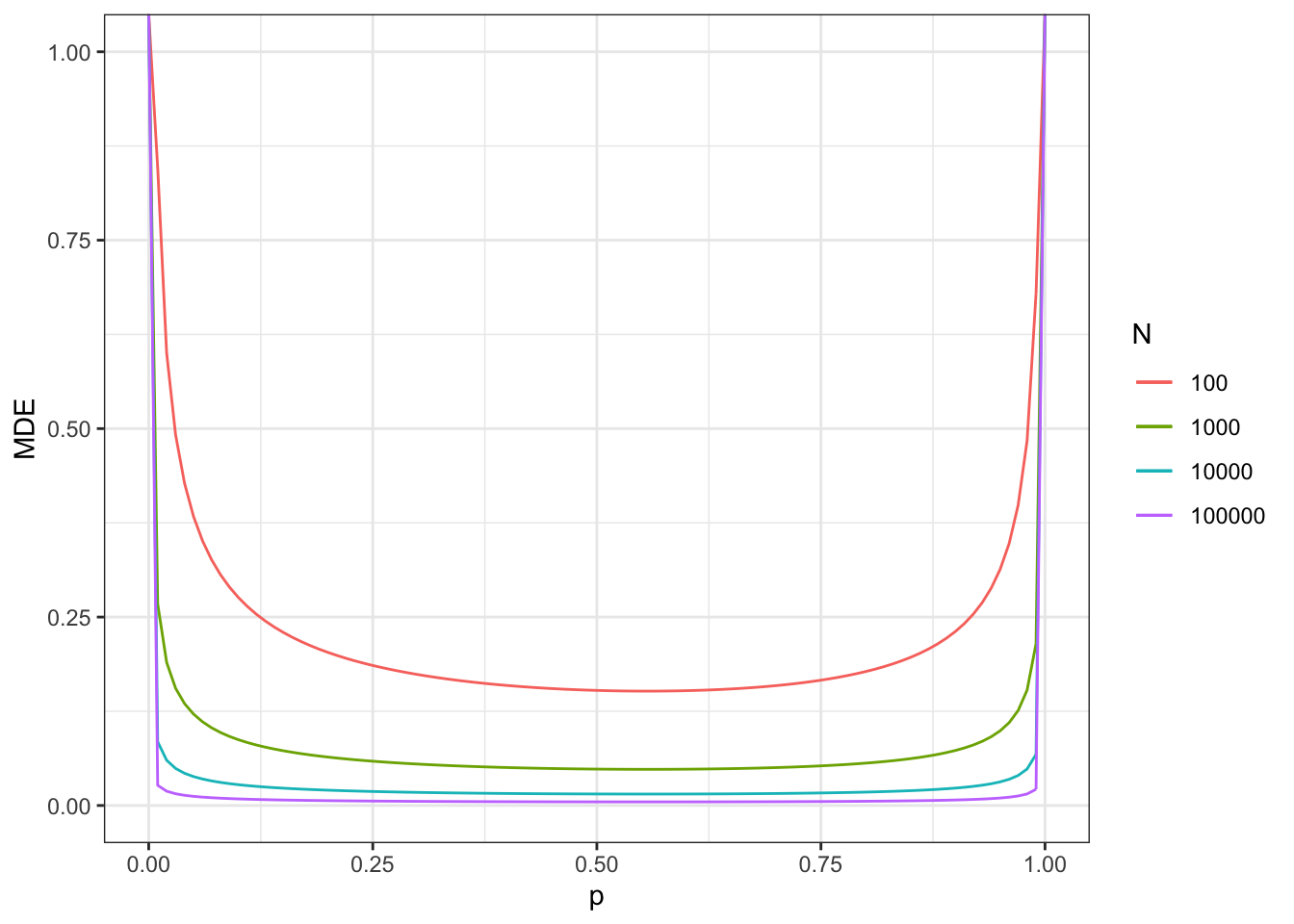
Figure 7.11: Minimum detectable effect for the 2 periods, 2 groups DID design in panel data
The actual proportion of treated in period 2 (vs never treated) is equal, in our sample, to 0.24.
With a sample size of \(N=100\), we reach a MDE of 0.19.
With a sample size of \(N=1000\), we reach a MDE of 0.06.
With a sample size of \(N=10000\), we reach a MDE of 0.02.
With a sample size of \(N=100000\), we reach a MDE of 0.006.
7.2.2.2.1.2 With repeated cross sections
In repeated cross sections, we can use Theorem 4.12 which says that:
\[\begin{align*} \sqrt{N}(\hat{\Delta}^Y_{DID_{cs}}-\Delta^Y_{DID}) & \stackrel{d}{\rightarrow} \mathcal{N}\left(0,\frac{\var{Y^0_{i,B}|D_i=0}}{(1-p)(1-p_A)} +\frac{\var{Y^0_{i,B}|D_i=1}}{p(1-p_A)}\right.\\ & \phantom{\stackrel{d}{\rightarrow}\mathcal{N}\left(0,\right.} \left. +\frac{\var{Y^0_{i,A}|D_i=0}}{(1-p)p_A} +\frac{\var{Y^1_{i,A}|D_i=1}}{pp_A}\right). \end{align*}\]
where \(p=\Pr(D_i=1)\) and \(p_A\) is the proportion of observations belonging to the After period. As a result, our estimate of \(C(\hat{\Delta}^Y_{DID_{cs}})\) in repeated cross sections is:
\[\begin{align*} \hat{C}(\hat{\Delta}^Y_{DID_{cs}}) & = \frac{\var{Y_{i,2}|D_i=1}}{pp_A}+ \frac{\var{Y_{i,1}|D_i=1}}{p(1-p_A)}+\frac{\var{Y_{i,2}|D_i=0}}{(1-p)p_A}+ \frac{\var{Y_{i,1}|D_i=0}}{(1-p)(1-p_A)}. \end{align*}\]
The corresponding functions in R are:
CE.DID.cs.fun <- function(p,pA,varY1b,varY0b,varY1a,varY0a){
  return((varY1a/(p*pA))+(varY0a/((1-p)*pA))+(varY1b/(p*(1-pA)))+(varY0b/((1-p)*(1-pA))))
}

MDE.DID.cs.fun <- function(p,pA,varY1b,varY0b,varY1a,varY0a,...){
  return(MDE(CE=CE.DID.cs.fun(p=p,pA=pA,varY1b=varY1b,varY0b=varY0b,varY1a=varY1a,varY0a=varY0a),...))
}
Example 7.9 Let us see how this formula works out in our example. We are going to keep the same sample and simply ignore the panel data dimension.
# estimating the variances
var.y.D.cs <- data %>%
            filter(time<=2,Ds==2 | Ds==99) %>%
            select(id,time,y,Ds) %>%
            group_by(time,Ds) %>%
            summarise(
              var.y = var(y)
            )
We can now compute the minimum detectable effect for various sample sizes and proportions of treated individuals, using \(\hatvar{y_{i,2}|D_i=1}=\) 0.27, \(\hatvar{y_{i,1}|D_i=1}=\) 0.19, \(\hatvar{y_{i,2}|D_i=0}=\) 0.38, and \(\hatvar{y_{i,1}|D_i=0}=\) 0.35. Let us finally check what Minimum Detectable Effect looks like as a function of \(p\) and of sample size, using \(p_A=0.5\).
Remark. In order to be fully comparable with the panel data case, we have to account for the fact that \(N\) in Theorem 4.12 is \(N\times T\) in Theorem 4.11. For that, we are going to multiply each entry of sample size in the MDE function by \(T=2\).
# pA
pA <- 0.5
Tmult  <- 2
# plot
ggplot() +
  xlim(0,1) +
  ylim(0,1) +
  geom_function(aes(color="100"),fun=MDE.DID.cs.fun,args=list(N=Tmult*100,pA=pA,varY1b=as.numeric(var.y.D.cs[1,3]),varY0b=as.numeric(var.y.D.cs[2,3]),varY1a=as.numeric(var.y.D.cs[3,3]),varY0a=as.numeric(var.y.D.cs[4,3]),alpha=alpha,kappa=kappa,oneside=FALSE)) +
  geom_function(aes(color="1000"),fun=MDE.DID.cs.fun,args=list(N=Tmult*1000,pA=pA,varY1b=as.numeric(var.y.D.cs[1,3]),varY0b=as.numeric(var.y.D.cs[2,3]),varY1a=as.numeric(var.y.D.cs[3,3]),varY0a=as.numeric(var.y.D.cs[4,3]),alpha=alpha,kappa=kappa,oneside=FALSE)) +
  geom_function(aes(color="10000"),fun=MDE.DID.cs.fun,args=list(N=Tmult*10000,pA=pA,varY1b=as.numeric(var.y.D.cs[1,3]),varY0b=as.numeric(var.y.D.cs[2,3]),varY1a=as.numeric(var.y.D.cs[3,3]),varY0a=as.numeric(var.y.D.cs[4,3]),alpha=alpha,kappa=kappa,oneside=FALSE)) +
  geom_function(aes(color="100000"),fun=MDE.DID.cs.fun,args=list(N=Tmult*100000,pA=pA,varY1b=as.numeric(var.y.D.cs[1,3]),varY0b=as.numeric(var.y.D.cs[2,3]),varY1a=as.numeric(var.y.D.cs[3,3]),varY0a=as.numeric(var.y.D.cs[4,3]),alpha=alpha,kappa=kappa,oneside=FALSE)) +
  scale_color_discrete(name="N") +
  ylab("MDE") +
  xlab("p") +
  theme_bw()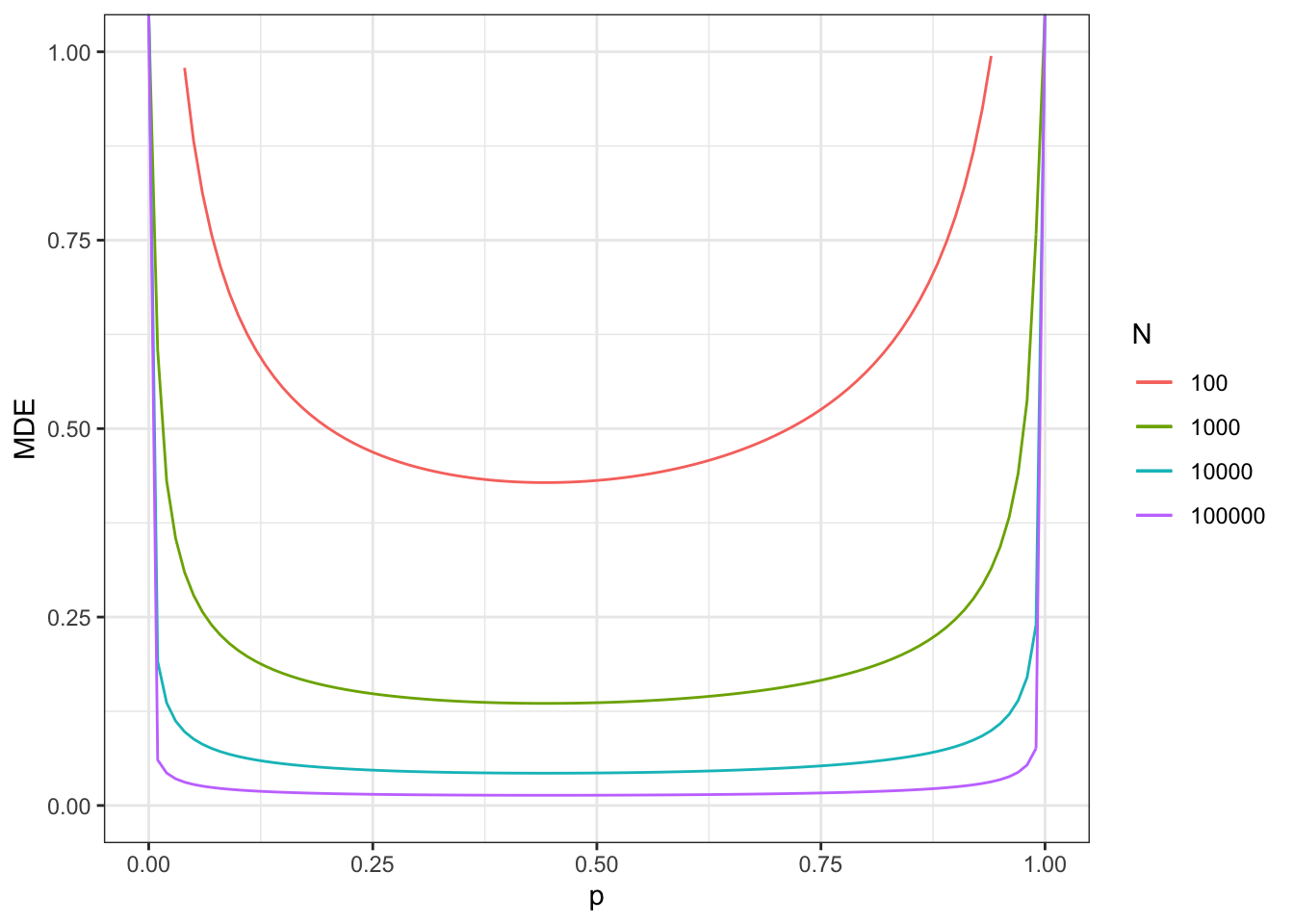
Figure 7.12: Minimum detectable effect for the 2 periods, 2 groups DID design in repeated cross sections
The actual proportion of treated in period 2 (vs never treated) is equal, in our sample, to 0.24.
With a sample size of \(N\times T=200\), we reach a MDE of 0.47.
With a sample size of \(N\times T=2000\), we reach a MDE of 0.15.
With a sample size of \(N\times T=20000\), we reach a MDE of 0.05.
With a sample size of \(N\times T=200000\), we reach a MDE of 0.015.
7.2.3 Power Analysis for Observational Methods
Power analysis for observational methods can be based on the results of Theorems 5.4 or 5.8. Let us start with the first one:
\[\begin{align*} \sqrt{N}(\hat\Delta^Y_{OLS(X)}-\Delta^Y_{TT}) & \stackrel{d}{\rightarrow} \mathcal{N}\left(0,\frac{\var{Y^0_i|X_i,D_i=0}}{1-\Pr(D_i=1)}+\frac{\var{Y^1_i|X_i,D_i=1}}{\Pr(D_i=1)}\right). \end{align*}\]
As a result, our estimate of \(C(\hat{\Delta}^Y_{OM})\) is:
\[\begin{align*} \hat{C}(\hat{\Delta}^Y_{OM}) & = \frac{\var{Y_{i}|X_i,D_i=0}}{1-\Pr(D_i=1)}+\frac{\var{Y_{i}|X_i,D_i=1}}{\Pr(D_i=1)}. \end{align*}\]
The corresponding functions in R are:
CE.OM.fun <- function(p,varY1bX,varY0bX){
  return((varY1bX/p)+(varY0bX/(1-p)))
}

MDE.OM.fun <- function(p,varY1bX,varY0bX,...){
  return(MDE(CE=CE.OM.fun(p=p,varY1bX=varY1bX,varY0bX=varY0bX),...))
}
A key component to compute \(C(\hat{\Delta}^Y_{OM})\) is the variance of \(Y_{i}\) conditional on observed covariates.
Example 7.10 Let’s see how this works in our example. We are going to use the same dataset as the one for the fuzzy regression discontinuity design. In order to be able to implement the MDE estimator with observational methods, we need to have access to one date of selection into the treatment and one outcome observed without the treatment (to be credible that no treatment has been given yet). We use as treatment, the treatment decided in period \(3\), as outcomes, the ones observed in period \(2\) and as controls, the outcomes observed in period \(1\).
We need to estimate the variance of outcomes \(Y_{i,2}\) conditional on \(Y_{i,1}\) and \(D_i\). One way to do that is to regress \(Y_{i,2}\) on \(Y_{i,1}\) in both the treated and control groups, and then to compute the variance of the residuals. Let’s do just that.
# estimating the conditional variance
# putting the data in wide format
data.wide <- data %>%
            select(id,time,y,Ds) %>%
            pivot_wider(names_from = "time",values_from = "y",names_prefix = "y")

# in the treated group
regy2y1D1 <- lm(y2 ~ y1,data=filter(data.wide,Ds==3))
vary2y1D1 <- var(regy2y1D1$residuals)
# in the control group
regy2y1D0 <- lm(y2 ~ y1,data=filter(data.wide,Ds==99))
vary2y1D0 <- var(regy2y1D0$residuals)

# proportion of treated
p3 <- data %>% filter(time==3,Ds==3 | Ds==99) %>% summarize(pD3=mean(D)) %>% pull(pD3)
We can now compute the minimum detectable effect for various sample sizes and proportions of treated individuals, using \(\hatvar{y_{i,2}|y_{i,1},D_i=1}=\) 0.06 and \(\hatvar{y_{i,2}|y_{i,1},D_i=0}=\) 0.06. Let us finally check what Minimum Detectable Effect looks like as a function of \(p\) and of sample size.
# plot
ggplot() +
  xlim(0,1) +
  ylim(0,1) +
  geom_function(aes(color="100"),fun=MDE.OM.fun,args=list(N=100,varY1bX=vary2y1D1,varY0bX=vary2y1D0,alpha=alpha,kappa=kappa,oneside=FALSE)) +
  geom_function(aes(color="1000"),fun=MDE.OM.fun,args=list(N=1000,varY1bX=vary2y1D1,varY0bX=vary2y1D0,alpha=alpha,kappa=kappa,oneside=FALSE)) +
  geom_function(aes(color="10000"),fun=MDE.OM.fun,args=list(N=10000,varY1bX=vary2y1D1,varY0bX=vary2y1D0,alpha=alpha,kappa=kappa,oneside=FALSE)) +
  geom_function(aes(color="100000"),fun=MDE.OM.fun,args=list(N=100000,varY1bX=vary2y1D1,varY0bX=vary2y1D0,alpha=alpha,kappa=kappa,oneside=FALSE)) +
  scale_color_discrete(name="N") +
  ylab("MDE") +
  xlab("p") +
  theme_bw()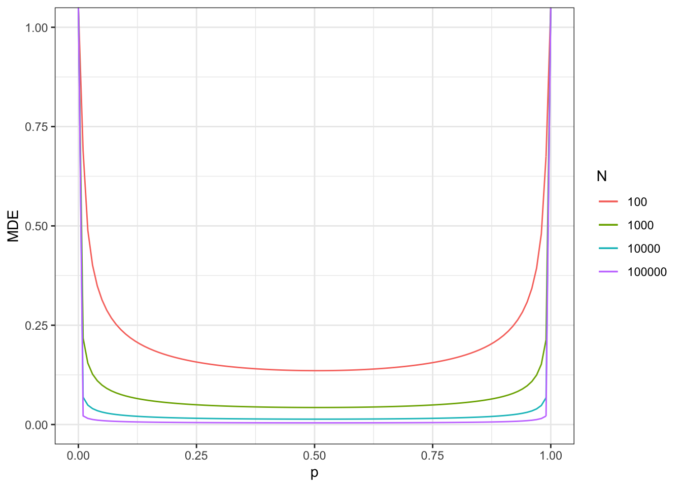
Figure 7.13: Minimum detectable effect of observational methods
The actual proportion of treated (vs never treated) is equal, in our sample, to 0.31.
With a sample size of \(N=100\), we reach a MDE of 0.15.
With a sample size of \(N=1000\), we reach a MDE of 0.05.
With a sample size of \(N=10000\), we reach a MDE of 0.01.
With a sample size of \(N=100000\), we reach a MDE of 0.005.
7.3 Limitations of and alternatives to traditional power analysis
Up to now, we have focused on traditional power analysis. There are several limitations with that approach that we are going to detail before describing two alternative approaches. What is fun is the alternative approaches I propose can be related to traditional power analysis ex-post and give rise to the same interpretations.
7.3.1 Limitations of traditional power analysis
Traditional power analysis suffers from several limitations that we are going to detail here.
7.3.1.1 Traditional power analysis favors publication bias
Traditional power analysis is based on Null Hypothesis Significance Testing (NHST): we assume that we are going to use a test for deciding whether the treatment effect of interest is significantly different from zero or not. NHST contributes to publication bias (see Chapter 13): by putting emphasis on results that are statistically significant, NHST contributes to populate the published record with an over-representation of statistically significant results. Since significant effects are larger than the average effect, summaries of the published record using meta-analysis will over-estimate the effect of programs, sometimes severely. Eschewing NHST, including when conducting power analysis, is one of the many ways to curb publication bias.
Remark. This is my own position on this and it is not shared widely. My priority is for users of statistical tools to focus on the order of magnitude of sampling noise, not on the position of a noisy measurement (a treatment effect estimate) relative to an arbitrary threshold. Of course, other tools are needed to get rid of publication bias, among registered reports, and they are detailed in Chapter 13.
7.3.1.2 With default settings, traditional power analysis has a very low signal to noise ratio
One of my main issues with traditional power analysis is that, with its basic settings that everyone uses, it actually settles on a very low value for the signal to noise ratio. Let me show you why. Let’s take \(2\epsilon\) as our measure of sampling noise, with \(2\epsilon=2\Phi^{-1}\left(\frac{\delta+1}{2}\right)\var{\hat{E}}\), following Assumption 7.1, with \(\delta\) the confidence level used to build the confidence interval. Let’s use \(\beta_A\) as our measure of the size of the treatment effect, which seems a good idea: it is the value of the treatment effect which seems ex ante most likely. Then we have:
Theorem 7.4 (Signal to Noise Ratio of Traditional Power Analysis) With \(\hat{E}\) complying with Assumption 7.1, for a one-sided test of size \(\alpha\) and power \(\kappa\), with a minimum detectable effect of \(\beta_A\), we have:
\[\begin{align*} \frac{\beta_A}{2\epsilon} & \approx \frac{\left(\Phi^{-1}\left(\kappa\right)+\Phi^{-1}\left(1-\alpha\right)\right)} {2\Phi^{-1}\left(\frac{\delta+1}{2}\right)} \end{align*}\]
Proof. Using Theorems 7.2 and Definition 2.1, we have:
\[\begin{align*} \frac{\beta_A}{2\epsilon} & \approx \frac{\left(\Phi^{-1}\left(\kappa\right)+\Phi^{-1}\left(1-\alpha\right)\right)\sqrt{\var{\hat{E}}}} {2\Phi^{-1}\left(\frac{\delta+1}{2}\right)\sqrt{\var{\hat{E}}}} \\ & = \frac{\left(\Phi^{-1}\left(\kappa\right)+\Phi^{-1}\left(1-\alpha\right)\right)} {2\Phi^{-1}\left(\frac{\delta+1}{2}\right)} \end{align*}\]
Remark. For a two-sided test, simply replace \(\alpha\) by \(\frac{\alpha}{2}\) in the formula of Theorem 7.4.
Theorem 7.4 shows that the signal to noise ratio of traditional approach power analysis is independent of \(\var{\hat{E}}\), the precision of the estimator. The signal to noise ratio will always be the same, whatever the precision of the estimator. This is a very strange property: it means that if we follow the advice of traditional power analysis, we will never have an incentive to increase the signal to noise ratio. This could very well not be a problem if the signal to noise ratio implied by traditional power analysis with its default settings (\(\alpha=0.05\) and \(\kappa=0.80\)) was large. What is its size in practice? Let’s compute it. In order to so, let’s define first a function which will compute the signal to noise ratio of traditional power analysis.
# functino computing signal to noise ratio
signal.to.noise <- function(alpha,kappa,delta,oneside=FALSE){
  if (oneside==TRUE){
    StoN <- (qnorm(kappa)+qnorm(1-alpha))/(2*qnorm((delta+1)/2))
  }
  if (oneside==FALSE){
    StoN <- (qnorm(kappa)+qnorm(1-alpha/2))/(2*qnorm((delta+1)/2))
  }
  return(StoN)
}
With the basic settings of traditional power analysis (\(\alpha=0.05\) and \(\kappa=0.80\)) and with \(\delta=0.95\), we thus have a signal to noise ratio equal to 0.63 with a one-sided test and to 0.71 with a two-sided test. With the same basic settings and \(\delta=0.99\), we have a signal to noise ratio of 0.48 with a one-sided test and to 0.54 with a two-sided test.
So, depending on how we define sampling noise and on the details of the power analysis, traditional power analysis gives rise to estimates with a signal to noise ratio between 0.5 and 0.7. A signal to noise ratio of 0.5 to 0.7 is very imprecise. It means that we accept a procedure which gives us, routinely, estimates of treatment effects where the signal (the treatment effect) is equal to 50% to 70% of the sampling noise.
Physicists like to express their estimates as multiples of \(\sigma=\sqrt{\var{\hat{E}}}\), the standard error of the estimated treatment effect. Using the proof of Theorem 7.4, we can show that \(\beta_A=\frac{\beta_A}{2\epsilon}2\Phi^{-1}\left(\frac{\delta+1}{2}\right)\sigma\), with traditional power analysis. When \(\frac{\beta_A}{2\epsilon}=0.5\), as with the default settings of traditional power analysis, we have \(\beta_A=\Phi^{-1}\left(\frac{\delta+1}{2}\right)\sigma\), that is \(\beta_A=\) 2.58 \(\sigma\) with \(\delta=0.99\) and \(\beta_A=\) 1.96 \(\sigma\) with \(\delta=0.95\). So we operate at levels of 2 to 2.5 \(\sigma\), whereas physicists like to operate at \(5\sigma\), that is at levels of precision at least twice as large.
How could we reach levels of precision similar to the ones the physicists use? One way would be to require a lower \(\alpha\) as a default setting of power analysis. Using \(\alpha=0.01\) for example gives rise to signal to noise ratios of 0.81 with a one-sided test and to 0.87 with a two-sided test \(\delta=0.95\) and to 0.61 with a one-sided test and to 0.66 with a two-sided test and \(\delta=0.99\). These are insufficient to reach the required precision. Indeed, we are at precision levels of \(\beta_A=\) 3.42 \(\sigma\) with \(\delta=0.99\) and \(\beta_A=\) 3.42 \(\sigma\) with \(\delta=0.95\). If we set \(\kappa=0.95\), we will be operating in precision levels that are closer to the pysicists’ one: \(\beta_A=\) 4.22 \(\sigma\) with \(\delta=0.99\) and \(\beta_A=\) 4.22 \(\sigma\) with \(\delta=0.95\).
Remark. All of this analysis is not to say that we should change our default settings for power analysis to \(\alpha=0.01\) and \(\kappa=0.95\). The sample size requirements for this settings might be daunting. In the absence of publication bias, running small experiments is fine since we aim to learn from their aggregation in a meta-analysis and not from any single study.
7.3.1.3 Traditional power analysis is complex
Traditional power analysis is not easy to understand and it is actually even harder to communicate to research partners. I once tried to explain the results of our power computations to a partner in the policy sphere. She could not understand the concept of minimum detectable effect. This idea that you’re postulating an effect that you will be able to detect with 80% chance was very weird to her. In our application (as is the case in a lot of applications), we did not have much choice on sample size. The most important thing she was trying to get was the threshold effect above which we would detect statistically significant estimates at the usual rates (5% for a two-sided t-test). She kept asking me for the minimum effect we needed to find that will be deemed different from zero. After thinking about it, I decided to communicate that effect to her, because she was correct in that the success of an intervention is generally measured in terms of statistical significance (much to my chagrin, as will be detailed in Chapter 13). Her requirement actually made a lot of sense, knowing the way statistical testing is used in practice.
Remark. In order to find the minimum effect that will trigger a statistically significant result, you can use the formulae in Theorem 7.2 by replacing \(\Phi^{-1}\left(\kappa\right)\) by zero.
A related issue with traditional power analysis is that it requires to specify a lot of different parameters. For example, in order to spit out a required sample size, you need to choose the size of the test \(\alpha\), whether it is one-sided or two-sided, its power \(\kappa\) and the MDE you’re trying to detect (or the most plausible effect size ex-ante). In general, researchers and practitioners have no idea how to choose these parameters or how to tailor them to their needs. That is why they rely on default settings most of the time, which gives rise to low precision and signal to noise ratios.
7.3.1.4 Traditional power analysis requires a closed form formula for sampling noise
A final limitation of traditional power analysis is that it only applies to estimators that comply with Assumption 7.1: they need to be asymptotically normal and we need to know their asymptotic distribution. That is why I spent a lot of time deriving these closed form formulae when I introduced the properties of each method. Most of these closed form formula do not exist in the literature, but without them, you cannot run traditional power analysis. The problem is that some estimators might not be asymptotically normally distributed or we might not be able to derive the features of their asymptotic distribution. What to do in that case? Let’s see.
7.3.2 An alternative to traditional power analysis
The alternative that I propose to traditional power analysis rests on two pillars. Let’s review them before studying three ways to implement them in practice.
7.3.2.1 The first pillar: choosing the level of sampling noise directly
I propose to eschew the use of NHST and to focus instead on quantifying sampling noise and the sample size required to reach a given level of precision. This has several advantages. First, we have much less parameters to set. For a given sample size, we can directly estimate the corresponding level of sampling noise. For a given target level of sampling noise, we can directly compute the sample size required to reach it. Second, by eschewing NHST, we also help to focus on the size of sampling noise, a qualitative measure, and not on the position of the estimated effect relative to an arbitrarily set threshold. Third and finally, our approach does not set the signal to noise ratio in stone. It only focuses on the size of sampling noise and leaves completely unspecified the likely size of the effect. In a sense, it asks the researcher and her partners what is the level of noise that they are comfortable with. If the funds are limited and sample size cannot be increased by much, my proposal makes it clear which type precision of we can expect.
In practice, the user of my proposal selects a level of sampling noise, either by specifying \(2\epsilon\) or simply \(\epsilon\), and recovers the required sample size. The user can alternatively select a given sample size \(N\) and recover the implied sampling noise (either \(2\epsilon\) or \(\epsilon\)). I tend to prefer using \(\epsilon\) as a measure of sampling noise since it can be put on the same level as the treatment effect itself by using \(\pm\epsilon\) to present precision. But this is a matter of taste, and using \(2\epsilon\) is also fine
Under Assumption 7.1, we can derive the sampling noise for a given sample size and the required sample size to reach a given level of sampling noise if we have an asymptotically normal estimator:
Theorem 7.5 (Alternative to Traditional Power Analysis) With \(\hat{E}\) complying with Assumption 7.1, we have:
\[\begin{align*} 2\epsilon & = 2\Phi^{-1}\left(\frac{\delta+1}{2}\right)\sqrt{\var{\hat{E}}}\\ N & = 4\left(\Phi^{-1}\left(\frac{\delta+1}{2}\right)\right)^2\frac{C(\hat{E})}{(2\epsilon)^2}, \end{align*}\]
with \(\var{\hat{E}}=\frac{C(\hat{E})}{N}\).
Example 7.11 Let’s see how Theorem 7.5 works in practice. We are going to focus on the case of the brute force randomized controlled trial, but the approach works similarly with all the other estimators we have examined above. Let us first generate some data:
param <- c(8,.5,.28,1500,0.9,0.01,0.05,0.05,0.05,0.1)
names(param) <- c("barmu","sigma2mu","sigma2U","barY","rho","theta","sigma2epsilon","sigma2eta","delta","baralpha")set.seed(1234)
N <-1000
mu <- rnorm(N,param["barmu"],sqrt(param["sigma2mu"]))
UB <- rnorm(N,0,sqrt(param["sigma2U"]))
yB <- mu + UB
YB <- exp(yB)
Ds <- rep(0,N)
Ds[YB<=param["barY"]] <- 1
epsilon <- rnorm(N,0,sqrt(param["sigma2epsilon"]))
eta<- rnorm(N,0,sqrt(param["sigma2eta"]))
U0 <- param["rho"]*UB + epsilon
y0 <- mu + U0 + param["delta"]
alpha.i <- param["baralpha"]+ param["theta"]*mu + eta
y1 <- y0+alpha.i
Y0 <- exp(y0)
Y1 <- exp(y1)
# randomized allocation of 50% of individuals
Rs <- runif(N)
R <- ifelse(Rs<=.5,1,0)
y <- y1*R+y0*(1-R)
Y <- Y1*R+Y0*(1-R)Let us now compute the required sample size to reach a given precision level \(\epsilon\).
# basic formulas
sample.size.alt <- function(epsilon,CE,delta){
    N <- 4*(qnorm((delta+1)/2)^2)*CE/(2*epsilon)^2
  return(round(N))
}
epsilon.alt <- function(N,CE,delta){
  epsilon <- qnorm((delta+1)/2)*sqrt(CE/N)
  return(epsilon)
}

# formulas for the BF design
sample.size.alt.BF.fun <- function(p,varYb,...){
  return(sample.size.alt(CE=CE.BF.fun(p=p,varYb=varYb),...))
}

epsilon.alt.BF.fun <- function(p,varYb,...){
  return(epsilon.alt(CE=CE.BF.fun(p=p,varYb=varYb),...))
}
Let us now plot the sample size as a function of the required precision in the brute force design for several values of \(p\):
ggplot() +
  xlim(0,1) +
  ylim(0,100000) +
  geom_function(aes(color="0.5"),fun=sample.size.alt.BF.fun,args=list(p=0.5,varYb=var(yB),delta=0.99)) +
  geom_function(aes(color="0.25"),fun=sample.size.alt.BF.fun,args=list(p=0.25,varYb=var(yB),delta=0.99)) +
  geom_function(aes(color="0.1"),fun=sample.size.alt.BF.fun,args=list(p=0.1,varYb=var(yB),delta=0.99)) +
  scale_color_discrete(name="p") +
  ylab("N") +
  xlab(expression(epsilon)) +
  scale_y_continuous(trans=log10_trans())+
  theme_bw()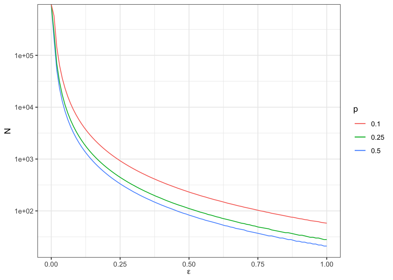
Figure 7.14: Required sample size for a given level of precision for the Brute Force design
As we can see from Figure 7.14, in order to reach a precision level of \(\pm 0.5\) with \(p=0.5\), we need a sample size of 83. To reach a precision level of \(\pm 0.2\) with \(p=0.5\), we need a sample size of 521. To reach a precision level of \(\pm 0.1\) with \(p=0.5\), we need a sample size of 2083. To reach a precision level of \(\pm 0.02\) with \(p=0.5\), we need a sample size of 5.2079^{4}.
7.3.2.2 The second pillar: simulating treatment allocation
Relying on Theorem 7.5 to implement my proposed approach solves several issues with traditional power analysis, but it still relies on the existence of an asymptotically normal approximation to sampling noise. The second pillar of my proposed approach uses randomly selected sample(s) as a way to estimate sampling noise without resorting to the closed form of an asymptotically normal approximation. I propose to use two distinct approaches: either using one unique random sample or using multiple random samples. Let’s detail these approaches in turn.
7.3.2.2.1 Power analysis using one random sample
This approach works well when we have a correct estimator of the sampling noise of our treatment effect but we have not derived its closed form in our particular case, or we have but we do not want to use it because it is too intricate or some components are too difficult to compute. This is the case for example when we use heteroskedasticity-robust standard errors without deriving how they apply to a treatment setting. This approach applies well when we have clustering as well, since most statistical software are able to account for clustering for most estimators, but we generally have not derived the precise formulae in a treatment effect context.
In practice, the proposed approach works as follows:
- We resample the baseline data (with replacement) in order to obtain the target sample size.
- We allocate the treatment among units as if we were actually implementing the actual selection rule.
- We estimate the treatment effect \(\hat{E}\) using the estimator \(E\) and recover its standard error \(\sqrt{\var{\hat{E}}}\).
- We use our estiamte of \(\sqrt{\var{\hat{E}}}\) in order to compute an estimate of \(\epsilon\) (using Theorem 7.5) or an estimate of MDE (using Theorem 7.2).
As a consequence, this approach works either with traditional power analysis (it uses a regression to estmate the sandard error instead of the closed form formula) or with my own proposal.
Remark. If the survey is clustered or stratified, step 1 above has to account for that. If the treatment allocation is clustered or stratified, both step 2 and step 3 have to account for that.
Example 7.12 Let us see how this approach works in our example. I am going to focus again on the brute force design, but there is a lot to learn by using the same approach for other designs and estimators. Let us first write a function that resamples the available data with replacement and then that computes the MDE (for the traditional approach to power analysis) and sampling noise \(\epsilon\) (for my proposed approach).
MDE.indirect.BF <- function(N.simul,y,p,alpha,kappa,delta,...){
  set.seed <- 1234
  resample <- sample(length(y),N.simul,replace=TRUE)
  y.simul <- y[resample]
  # randomized allocation of 50% of individuals
  Rs.simul <- runif(N.simul)
  R.simul <- ifelse(Rs.simul<=p,1,0)
  reg.ols.ww.bf.simul <- lm(y.simul~R.simul)
  varE.simul <- vcovHC(reg.ols.ww.bf.simul,type='HC2')[2,2]
  MDE.simul <- MDE.var(alpha=alpha,kappa=kappa,varE=varE.simul,...)
  epsilon.simul <- epsilon.alt(N=N.simul,CE=varE.simul*N.simul,delta=delta)
  results <- c(MDE.simul,epsilon.simul)
  names(results) <- c('MDE_simul','Epsilon_simul')
  return(results)
}

# computations
p<- 0.5
test.indirect <- as.data.frame(t(sapply(N.sample,MDE.indirect.BF,alpha=0.05,kappa=0.8,y=y,p=p,delta=0.99,oneside=FALSE)))
test.indirect$N.simul <- N.sample

# adding results of traditional approach for comparison
test.indirect$MDE_tradi <-sapply(N.sample,MDE.BF.fun,p=p,varYb=var(yB),alpha=0.05,kappa=0.8,oneside=FALSE)
test.indirect$Epsilon_tradi <-sapply(N.sample,epsilon.alt.BF.fun,p=p,varYb=var(yB),delta=0.99)

# putting results in long form to enable plotting
test.indirect.long <- test.indirect %>%
                        pivot_longer(cols=!N.simul,names_to=c('Type','Method'),names_sep=c("_"),values_to='Estimate') %>%
                        mutate(
                          Type=factor(Type,levels=c('MDE','Epsilon')),
                          Method=recode_factor(Method,"simul"="Simulation","tradi"="Traditional"),
                          Method=factor(Method,levels=c('Traditional','Simulation'))
) ggplot(test.indirect.long, aes(x=as.factor(N.simul), y=Estimate, fill=Method)) +
geom_bar(position=position_dodge(), stat="identity") +
xlab("Sample Size") +
theme_bw()+
facet_grid(.~Type)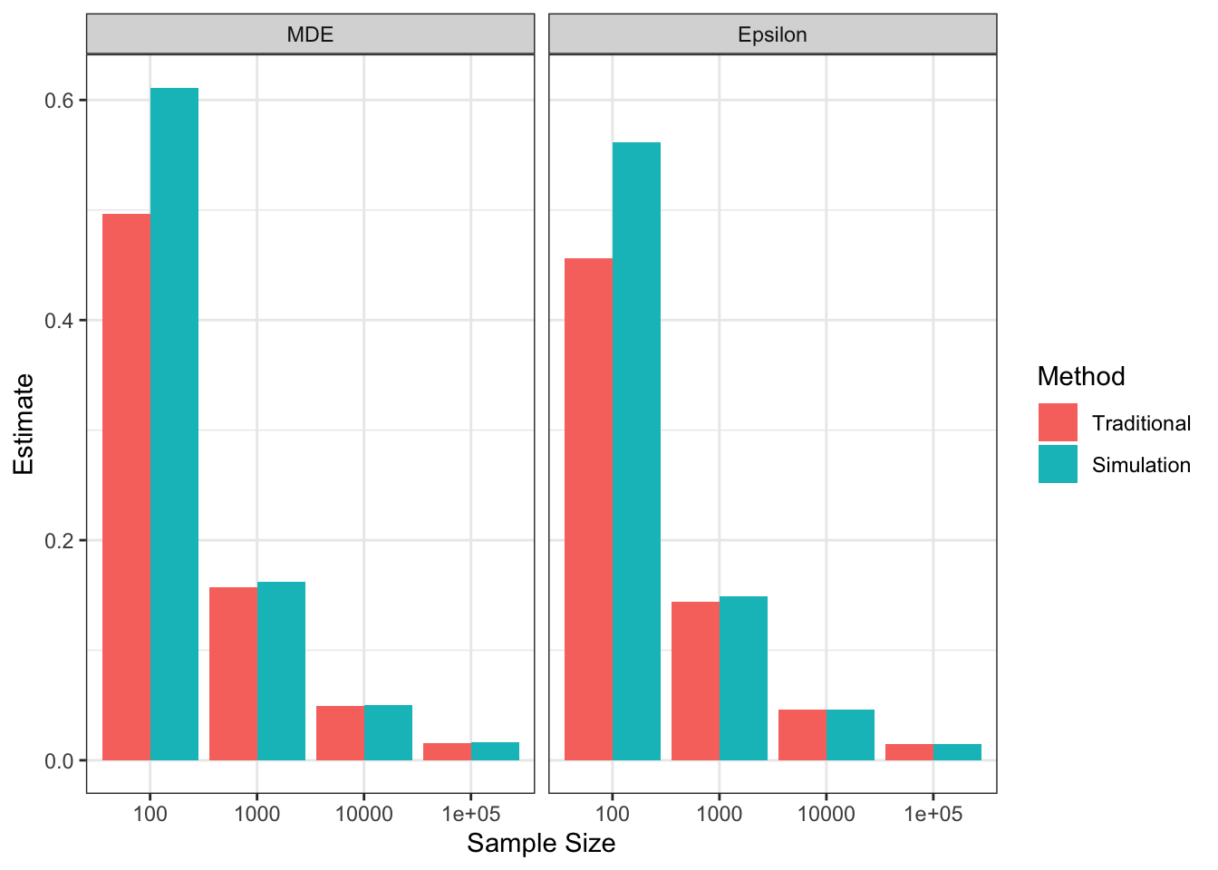
Figure 7.15: MDE, and sample size for the Brute Force design using traditional and novel power analysis
What is pretty cool is that both approaches find very similar results for both MDE and \(\epsilon\). What is less expected is that actually MDE and \(\epsilon\) are extremely similar, although they relate to profoundly different concepts: MDE refers to a minimum effect size for detection using NHST with \(\alpha=0.05\) and \(\kappa=0.80\) while \(\epsilon\) refers to the sampling noise to be expected with a given sample size for \(\delta=0.99\). Why does the measure of sampling noise stemming out of my proposed approach ends up being so close to the measure of minimum detectable effect stemming from the traditional approach? Well, this does make sense once you examine the formulae for both terms in Theorems 7.2 and 7.5: both MDE and \(\epsilon\) depend on \(\sqrt{\var{\hat{E}}}\). The formula for MDE multiplies \(\sqrt{\var{\hat{E}}}\) by \(\Phi^{-1}\left(\kappa\right)+\Phi^{-1}\left(1-\frac{\alpha}{2}\right)\) (in the two-sided case) while the formula for \(\epsilon\) multiplies \(\sqrt{\var{\hat{E}}}\) by \(\Phi^{-1}\left(\frac{\delta+1}{2}\right)\). What happens is that these two terms are extremely close to each other with the parameters we have chosen so far. With \(\alpha=0.05\) and \(\kappa=0.80\), the first term is equal to 2.8. With \(\delta=0.99\), the second term is equal to 2.58.
Overall, my feeling is that even if the results of two approaches are miraculously similar, they have completely different implications. The traditional approach basically amounts to say that, when you estimate an effect \(\beta_A\pm\epsilon\), it is perfectly fine (and actually best practice) that \(\beta_A\) is of the same order of magnitude as \(\epsilon\). In the best case scenario where \(\delta=0.95\), \(\frac{\beta_A}{\epsilon}=\) 1.43 so that is \(\beta_A\) is 43% larger than \(\epsilon\). In the case where \(\delta=0.99\), \(\frac{\beta_A}{\epsilon}=\) 1.09 so that is \(\beta_A\) is only 33% larger than \(\epsilon\).
With the novel approach, you would probably find these settings appalling and utterly insufficient.
It means that you are accepting a situation in which \(\epsilon\) is barely smaller than \(\beta_A\).
You are in a \(2\sigma\) world.
The signal to noise ratio is well below one (\(\frac{\beta_A}{2\epsilon}=\) 0.71 with \(\delta=0.95\) and 0.54 with \(\delta=0.99\)).
This is a situation in which you have a 20% chance of not detecting the true effect if it has size \(\beta_A\).
20%!
Why even run the experiment in that case?
I’d be much more comfortable with a 1% to 5% chance.
With these settings, you are adding 0.8 to 1.48 \(\sigma\) to your precision.
But, even deeper, my proposed approach wants you to stop thinking about probabilities of detection. Just think about noise. Are you fine with an uncertainty of \(\pm\epsilon\) around your main estimate? Does it make sense for you to run this experiment? If you have no choice (that is sample size has been chosen and the experiment will run), my proposed approach tells you simply that \(\pm\epsilon\) is the best you can do and that you have to live with it. Maybe it will be insufficient for now, but publishing this result and collecting similar ones will get us closer and closer to the truth.
7.3.2.2.2 Power analysis using randomization inference
One final limitation of the previous approach is that it is only valid when we have an estimator of sampling noise that is already built-in out statistical software. What if we do not have such an estimator, or we do not know which one is correct? Well, here, it might help tremendously to use randomization inference. We are going to measure of much the treatment effect varies over randomized allocations of the treatment. This is going to be a good approximation of the magnitude of the sampling noise we will be facing in the real experiment.
Remark. One might want to associate ranoomization inference with the bootstrap. That is, draw a new sample with replacement each time you selevct a new treatment allocation. Not using the bootstrap will estimate sampling noise for the sample average treatment effect, while combining the bootstrap with randomization inference will estimate sampling noise for the population treatment effect.
Example 7.13 Let’s see how this approach works in our example. Let’s write the code to produce a randomization inference estimate.
# treatment effect estimate for one randomized sample
MDE.indirect.BF.RI <- function(seed,N.simul,y,p,alpha,kappa,delta,...){
  set.seed(seed)
  resample <- sample(length(y),N.simul,replace=TRUE)
  y.simul <- y[resample]
  # randomized allocation of 50% of individuals
  Rs.simul <- runif(N.simul)
  R.simul <- ifelse(Rs.simul<=p,1,0)
  reg.ols.ww.bf.simul <- lm(y.simul~R.simul)
  estim.RI <- reg.ols.ww.bf.simul$coefficients[[2]]
  return(estim.RI)
}

simuls.MDE.indirect.BF.RI <- function(Nsim,...){
  MDE.indirect.BF.RI.N <- unlist(lapply(1:Nsim,MDE.indirect.BF.RI,...))
  return(MDE.indirect.BF.RI.N)
}

sf.simuls.MDE.indirect.BF.RI <- function(Nsim,...){
  sfInit(parallel=TRUE,cpus=2*ncpus)
  MDE.indirect.BF.RI.N <- unlist(sfLapply(1:Nsim,MDE.indirect.BF.RI,...))
  sfStop()
  return(MDE.indirect.BF.RI.N)
}

Nsim <- 1000
#Nsim <- 10
N.sample <- c(100,1000,10000,100000)
#N.sample <- c(100,1000,10000)
#N.sample <- c(100,1000)
#N.sample <- c(100)

simuls.sampling.noise.BF.RI <-  matrix(unlist(lapply(N.sample,sf.simuls.MDE.indirect.BF.RI,Nsim=Nsim,y=y,p=0.5,alpha=0.05,kappa=0.8,delta=0.99,oneside=FALSE)),ncol=length(N.sample),nrow=Nsim,byrow = FALSE)
## R Version: R version 4.1.1 (2021-08-10)Let’s plot the resulting estimates:
par(mfrow=c(2,2))
for (i in 1:length(N.sample)){
  hist(simuls.sampling.noise.BF.RI[[i]],breaks=30,main=paste('N=',as.character(N.sample[i])),xlab=expression(hat(Delta^y)[WW]),xlim=c(-0.55,0.55))
}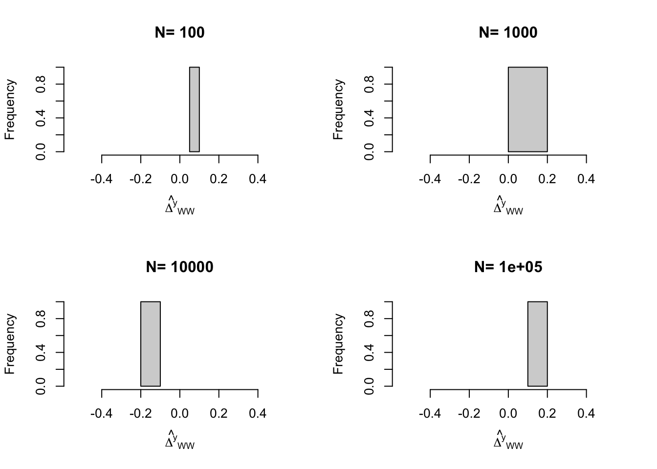
Figure 7.16: Distribution of the Brute Force estimator using randomization inference
And the resulting estimates of sampling noise:
# summary stat
simuls.sampling.noise.BF.RI.summary <- as.data.frame(simuls.sampling.noise.BF.RI) %>%
                                        pivot_longer(1:4,names_to="SampleSize",values_to="Estimate") %>%
                                        group_by(SampleSize) %>%
                                        summarize(
                                          Se = sqrt(var(Estimate))
                                        ) %>%
                                        mutate(
                                          TT = 0,
                                          SampleSize=as.numeric(SampleSize)
)ggplot(simuls.sampling.noise.BF.RI.summary, aes(x=as.factor(SampleSize), y=TT)) +
geom_pointrange(aes(ymin=TT-Se*1.96, ymax=TT+Se*1.96),color='red') +
xlab("Sample Size")+
theme_bw()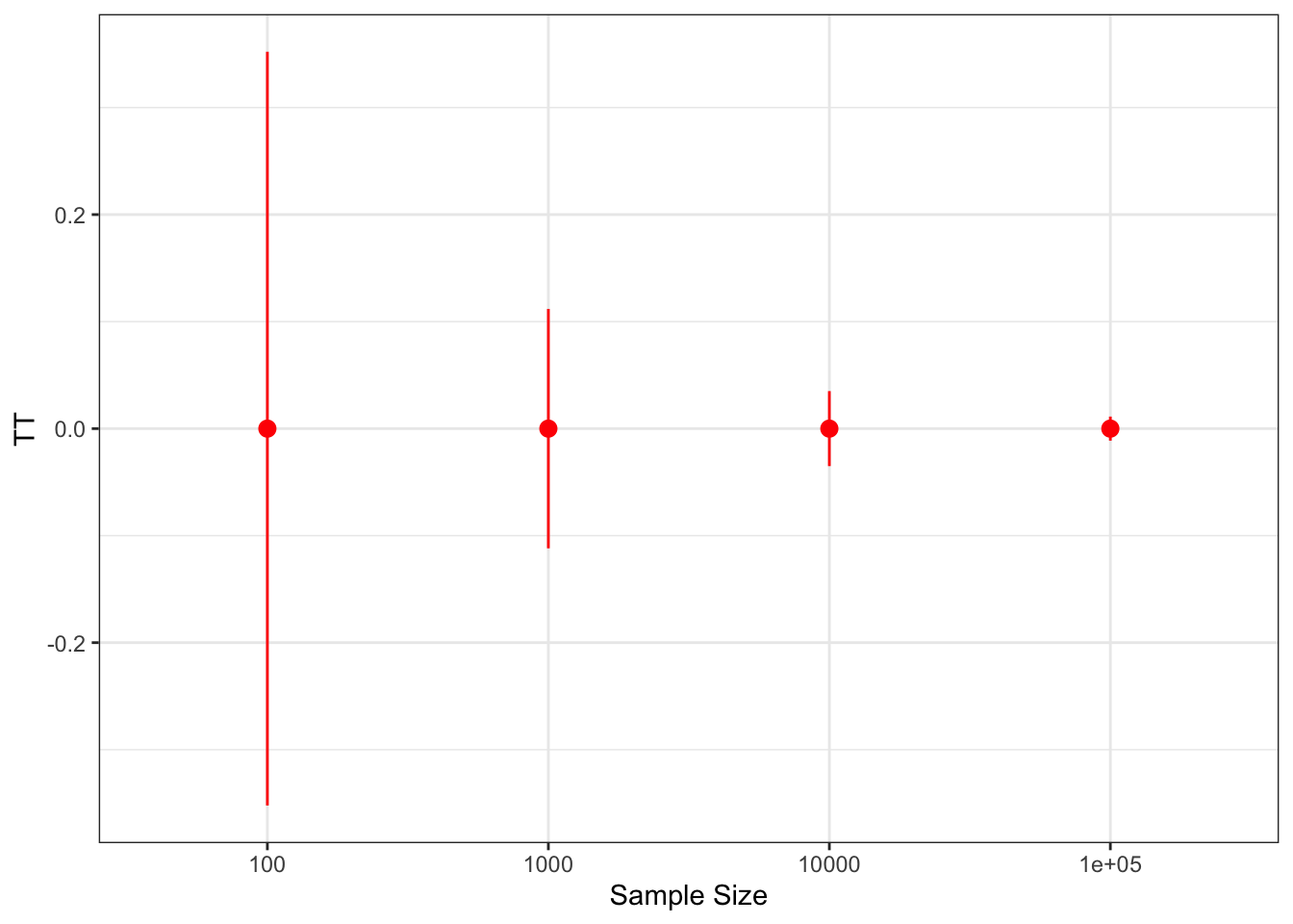
Figure 7.17: Sampling noise of the Brute Force estimator using randomization inference
We can also compare sampling noise estimated using randomization inference to the one estimated by using only one sample and the one estimated using the traditional approach.
# preparing the data
test.indirect <- test.indirect %>%
                  left_join(simuls.sampling.noise.BF.RI.summary,by=c('N.simul'='SampleSize')) %>%
                  rename(
                    Epsilon_RI=Se,
                    MDE_RI=TT
                  )%>%
                  mutate(
                    Epsilon_RI = qnorm((0.99+1)/2)*Epsilon_RI
                  )


# putting results in long form to enable plotting
test.indirect.long <- test.indirect %>%
                        pivot_longer(cols=!N.simul,names_to=c('Type','Method'),names_sep=c("_"),values_to='Estimate') %>%
                        mutate(
                          Type=factor(Type,levels=c('MDE','Epsilon')),
                          Method=recode_factor(Method,"simul"="Simulation","tradi"="Traditional","RI"="Randomization Inference"),
                          Method=factor(Method,levels=c('Traditional','Simulation',"Randomization Inference"))
                        )
Let’s plot the result:
ggplot(filter(test.indirect.long,Type=='Epsilon'), aes(x=as.factor(N.simul), y=Estimate, fill=Method)) +
  geom_bar(position=position_dodge(), stat="identity") +
  xlab("Sample Size") +
  theme_bw()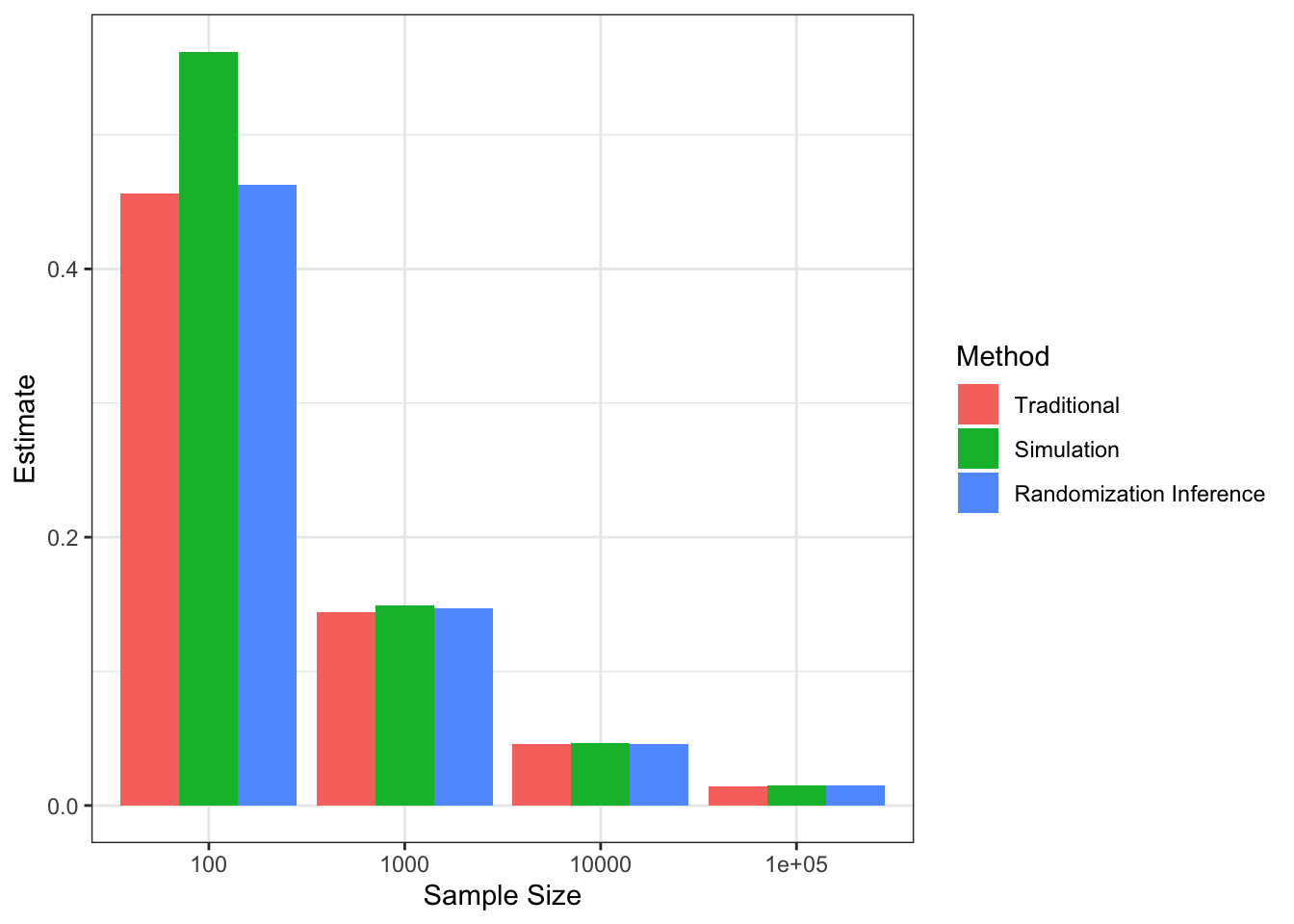
Figure 7.18: MDE, and sample size for the Brute Force design using traditional, one simulation and randomization inference for power analysis
We can see that our estimates of sampling noise using the various approaches are very similar, which is great.