Chapter 3 Randomized Controlled Trials
The most robust and rigorous method that has been devised by social scientists to estimate the effect of an intervention on an outcome is the Randomized Controlled Trial (RCT). RCTs are used extensively in the field to evaluate a wide array of programs, from development, labor and education interventions to environmental nudges to website and search engine features.
The key feature of an RCT is the introduction by the researcher of randomness in the allocation of the treatment. Individuals with \(R_i=1\), where \(R_i\) denotes the outcome of a random event, such as a coin toss, have a higher probability of receiving the treatment. Potential outcomes have the same distribution in both \(R_i=1\) and \(R_i=0\) groups. If we observe different outcomes between the treatment and control group, it has to be because of the causal effect of the treatment, since both groups only differ by the proportion of treated and controls.
The most attractive feature of RCTs is that researchers enforce the main identification assumption (we do not have to assume that it holds, we can make sure that it does). This property of RCTs distinguishes them from all the other methods that we are going to learn in this class.
In this lecture, we are going to study how to estimate the effect of an intervention on an outcome using RCTs. We are especially going to study the various types of designs and what can be recovered from them using which technique. For each design, we are going to detail which treatment effect it enables us to identify, how to obtain a sample estimate of this treatment effect and how to estimate the associated sampling noise. The main substantial difference between these four designs are the types of treatment effect parameters that they enable us to recover. Sections 3.1 to 3.4 of this lecture introduces the four designs and how to analyze them.
Unfortunately, RCTs are not bullet proof. They suffer from problems that might make their estimates of causal effects badly biased. Section ?? surveys the various threats and what we can do to try to minimize them.
3.1 Brute Force Design
In the Brute Force Design, eligible individuals are randomly assigned to the treatment irrespective of their willingness to accept it and have to comply with the assignment. This is a rather dumb procedure but it is very easy to analyze and that is why I start with it. With the Brute Force Design, you can recover the average effect of the treatment on the whole population. This parameter is generally called the Average Treatment Effect (ATE).
In this section, I am going to detail the assumptions required for the Brute Force Design to identify the ATE, how to form an estimator of the ATE and how to estimate its sampling noise.
3.1.1 Identification
In the Brute Force Design, we need two assumptions for the ATE to be identified in the population: Independence and Brute Force Validity.
Definition 3.1 (Independence) We assume that the allocation of the program is independent of potential outcomes: \[\begin{align*} R_i\Ind(Y_i^0,Y_i^1). \end{align*}\]
Here, \(\Ind\) codes for independence or random variables. Independence can be enforced by the randomized allocation.
We need a second assumption for the Brute Force Design to work:
Definition 3.2 (Brute Force Validity) We assume that the randomized allocation of the program is mandatory and does not interfere with how potential outcomes are generated: \[\begin{align*} Y_i & = \begin{cases} Y_i^1 & \text{ if } R_i=1 \\ Y_i^0 & \text{ if } R_i=0 \end{cases} \end{align*}\] with \(Y_i^1\) and \(Y_i^0\) the same potential outcomes as defined in Lecture~0 with a routine allocation of the treatment.
Under both Independence and Brute Force Validity, we have the following result:
Theorem 3.1 (Identification in the Brute Force Design) Under Assumptions 3.1 and 3.2, the WW estimator identifies the Average Effect of the Treatment (ATE): \[\begin{align*} \Delta^Y_{WW} & = \Delta^Y_{ATE}, \end{align*}\]
with: \[\begin{align*} \Delta^Y_{WW} & = \esp{Y_i|R_i=1} - \esp{Y_i|R_i=0} \\ \Delta^Y_{ATE} & = \esp{Y_i^1-Y_i^0}. \end{align*}\]
Proof. \[\begin{align*} \Delta^Y_{WW} & = \esp{Y_i|R_i=1} - \esp{Y_i|R_i=0} \\ & = \esp{Y^1_i|R_i=1} - \esp{Y^0_i|R_i=0} \\ & = \esp{Y_i^1}-\esp{Y_i^0}\\ & = \esp{Y_i^1-Y_i^0}, \end{align*}\] where the first equality uses Assumption 3.2, the second equality Assumption 3.1 and the last equality the linearity of the expectation operator.
Remark. As you can see from Theorem 3.1, ATE is the average effect of the treatment on the whole population, those who would be eligible for it and those who would not. ATE differs from TT because the effect of the treatment might be correlated with treatment intake. It is possible that the treatment has a bigger (resp. smaller) effect on treated individuals. In that case, ATE is higher (resp. smaller) than TT.
Remark. Another related design is the Brute Force Design among Eligibles. In this design, you impose the treatment status only among eligibles, irrespective of whether they want the treatment or not. It can be operationalized using the selection rule used in Section 3.2.
Example 3.1 Let’s use the example to illustrate the concept of ATE. Let’s generate data with our usual parameter values without allocating the treatment yet:
param <- c(8,.5,.28,1500,0.9,0.01,0.05,0.05,0.05,0.1)
names(param) <- c("barmu","sigma2mu","sigma2U","barY","rho","theta","sigma2epsilon","sigma2eta","delta","baralpha")set.seed(1234)
N <-1000
mu <- rnorm(N,param["barmu"],sqrt(param["sigma2mu"]))
UB <- rnorm(N,0,sqrt(param["sigma2U"]))
yB <- mu + UB
YB <- exp(yB)
Ds <- rep(0,N)
Ds[YB<=param["barY"]] <- 1
epsilon <- rnorm(N,0,sqrt(param["sigma2epsilon"]))
eta<- rnorm(N,0,sqrt(param["sigma2eta"]))
U0 <- param["rho"]*UB + epsilon
y0 <- mu + U0 + param["delta"]
alpha <- param["baralpha"]+ param["theta"]*mu + eta
y1 <- y0+alpha
Y0 <- exp(y0)
Y1 <- exp(y1)In the sample, the ATE is the average difference between \(y_i^1\) and \(y_i^0\), or – the expectation operator being linear – the difference between average \(y_i^1\) and average \(y_i^0\). In our sample, the former is equal to 0.179 and the latter to 0.179.
In the population, the ATE is equal to:
\[\begin{align*} \Delta^y_{ATE} & = \esp{Y_i^1-Y_i^0} \\ & = \esp{\alpha_i} \\ & = \bar{\alpha}+\theta\bar{\mu}. \end{align*}\]
Let’s write a function to compute the value of the ATE and of TT (we derived the formula for TT in the previous lecture):
delta.y.ate <- function(param){
  return(param["baralpha"]+param["theta"]*param["barmu"])
}
delta.y.tt <- function(param){
  return(param["baralpha"]+param["theta"]*param["barmu"]-param["theta"]*((param["sigma2mu"]*dnorm((log(param["barY"])-param["barmu"])/(sqrt(param["sigma2mu"]+param["sigma2U"]))))/(sqrt(param["sigma2mu"]+param["sigma2U"])*pnorm((log(param["barY"])-param["barmu"])/(sqrt(param["sigma2mu"]+param["sigma2U"]))))))
}
In the population, with our parameter values, \(\Delta^y_{ATE}=\) 0.18 and \(\Delta^y_{TT}=\) 0.172. In our case, selection into the treatment is correlated with lower outcomes, so that \(TT\leq ATE\).
In order to implement the Brute Force Design in practice in a sample, we simply either draw a coin repeatedly for each member of the sample, assigning for example, all “heads” to the treatment and all “tails” to the control. Because it can be a little cumbersome, it is possible to replace the coin toss by a pseudo-Random Number Generator (RNG), which is is an algorithm that tries to mimic the properties of random draws. When generating the samples in the numerical exmples, I actually use a pseudo-RNG. For example, we can draw from a uniform distribution on \([0,1]\) and allocate to the treatment all the individuals whose draw is smaller than 0.5:
\[\begin{align*} R_i^* & \sim \mathcal{U}[0,1]\\ R_i & = \begin{cases} 1 & \text{ if } R_i^*\leq .5 \\ 0 & \text{ if } R_i^*> .5 \end{cases} \end{align*}\]
The advantage of using a uniform law is that you can set up proportions of treated and controls easily.
Example 3.2 In our numerical example, the following R code generates two random groups, one treated and one control, and imposes the Assumption of Brute Force Validity:
# randomized allocation of 50% of individuals
Rs <- runif(N)
R <- ifelse(Rs<=.5,1,0)
y <- y1*R+y0*(1-R)
Y <- Y1*R+Y0*(1-R)Remark. It is interesting to stop for one minute to think about how the Brute Force Design solves the FPCI. First, with the ATE, the counterfactual problem is more severe than in the case of the TT. In the routine mode of the program, where only eligible individuals receive the treatment, both parts of the ATE are unobserved:
- \(\esp{Y_i^1}\) is unobserved since we only observe the expected value of outcomes for the treated \(\esp{Y_i^1|D_i=1}\), and they do not have to be the same.
- \(\esp{Y_i^0}\) is unobserved since we only observe the expected value of outcomes for the untreated \(\esp{Y_i^0|D_i=0}\), and they do not have to be the same.
What the Brute Force Design does, is that it allocates randomly one part of the sample to the treatment, so that we see \(\esp{Y_i^1|R_i=1}=\esp{Y_i^1}\) and one part to the control so that we see \(\esp{Y_i^0|R_i=0}=\esp{Y_i^0}\).
3.1.2 Estimating ATE
3.1.2.1 Using the WW estimator
In order to estimate ATE in a sample where the treatment has been randomized using a Brute Force Design, we simply use the sample equivalent of the With/Without estimator: \[\begin{align*} \hat{\Delta}^Y_{WW} & = \frac{1}{\sum_{i=1}^N R_i}\sum_{i=1}^N Y_iR_i-\frac{1}{\sum_{i=1}^N (1-R_i)}\sum_{i=1}^N Y_i(1-R_i). \end{align*}\]
Example 3.3 In our numerical example, the WW estimator can be computed as follows in the sample:
The WW estimator of the ATE in the sample is equal to 0.156. Let’s recall that the true value of ATE is 0.18 in the population and 0.179 in the sample.
We can also see in our example how the Brute Force Design approximates the counterfactual expectation \(\esp{y_i^1}\) and its sample equivalent mean \(\frac{1}{\sum_{i=1}^N}\sum_{i=1}^N y^1_i\) by the observed mean in the treated sample \(\frac{1}{\sum_{i=1}^N R_i}\sum_{i=1}^N y_iR_i\). In our example, the sample value of the counterfactual mean potential outcome \(\frac{1}{\sum_{i=1}^N}\sum_{i=1}^N y^1_i\) is equal to 8.222 and the sample value of its observed counterpart is 8.209. Similarly, the sample value of the counterfactual mean potential outcome \(\frac{1}{\sum_{i=1}^N}\sum_{i=1}^N y^0_i\) is equal to 8.043 and the sample value of its observed counterpart is 8.054.
3.1.2.2 Using OLS
As we have seen in Lecture 0, the WW estimator is numerically identical to the OLS estimator of a linear regression of outcomes on treatment: The OLS coefficient \(\beta\) in the following regression: \[\begin{align*} Y_i & = \alpha + \beta R_i + U_i \end{align*}\] is the WW estimator.
Example 3.4 In our numerical example, we can run the OLS regression as follows:
\(\hat{\Delta}^y_{OLS}=\) 0.156 which is exactly equal, as expected, to the WW estimator: 0.156.
3.1.2.3 Using OLS conditioning on covariates
The advantage of using OLS other the direct WW comparison is that it gives you a direct estimate of sampling noise (see next section) but also that it enables you to condition on additional covariates in the regression: The OLS coefficient \(\beta\) in the following regression: \[\begin{align*} Y_i & = \alpha + \beta R_i + \gamma' X_i + U_i \end{align*}\] is a consistent (and even unbiased) estimate of the ATE.
proof needed, especially assumption of linearity. Also, is interaction between \(X_i\) and \(R_i\) needed?
Example 3.5 In our numerical example, we can run the OLS regression conditioning on \(y_i^B\) as follows:
\(\hat{\Delta}^y_{OLSX}=\) 0.177. Note that \(\hat{\Delta}^y_{OLSX}\neq\hat{\Delta}^y_{WW}\). There is no numerical equivalence between the two estimators.
Remark. Why would you want to condition on covariates in an RCT? Indeed, covariates should be balanced by randomization and thus there does not seem to be a rationale for conditioning on potential confounders, since there should be none. The main reason why we condition on covariates is to decrease sampling noise. Remember that sampling noise is due to imbalances between confounders in the treatment and control group. Since these imbalances are not systematic, the WW estimator is unbiased. We can also make the bias due to these unbalances as small as we want by choosing an adequate sample size (the WW estimator is consistent). But for a given sample size, these imbalances generate sampling noise around the true ATE. Conditioning on covariates helps decrease sampling noise by accounting for imbalances due to observed covariates. If observed covariates explain a large part of the variation in outcomes, conditioning on them is going to prevent a lot of sampling noise from occuring.
Example 3.6 In order to make the gains in precision from conditioning on covariates apparent, let’s use Monte Carlo simulations of our numerical example.
monte.carlo.brute.force.ww <- function(s,N,param){
  set.seed(s)
  mu <- rnorm(N,param["barmu"],sqrt(param["sigma2mu"]))
  UB <- rnorm(N,0,sqrt(param["sigma2U"]))
  yB <- mu + UB
  YB <- exp(yB)
  Ds <- rep(0,N)
  Ds[YB<=param["barY"]] <- 1
  epsilon <- rnorm(N,0,sqrt(param["sigma2epsilon"]))
  eta<- rnorm(N,0,sqrt(param["sigma2eta"]))
  U0 <- param["rho"]*UB + epsilon
  y0 <- mu +  U0 + param["delta"]
  alpha <- param["baralpha"]+  param["theta"]*mu + eta
  y1 <- y0+alpha
  Y0 <- exp(y0)
  Y1 <- exp(y1)
  # randomized allocation of 50% of individuals
  Rs <- runif(N)
  R <- ifelse(Rs<=.5,1,0)
  y <- y1*R+y0*(1-R)
  Y <- Y1*R+Y0*(1-R)
  reg.y.R.ols <- lm(y~R)
  return(c(reg.y.R.ols$coef[2],sqrt(vcovHC(reg.y.R.ols,type='HC2')[2,2])))
}

simuls.brute.force.ww.N <- function(N,Nsim,param){
  simuls.brute.force.ww <- as.data.frame(matrix(unlist(lapply(1:Nsim,monte.carlo.brute.force.ww,N=N,param=param)),nrow=Nsim,ncol=2,byrow=TRUE))
  colnames(simuls.brute.force.ww) <- c('WW','se')
  return(simuls.brute.force.ww)
}

sf.simuls.brute.force.ww.N <- function(N,Nsim,param){
  sfInit(parallel=TRUE,cpus=2*ncpus)
  sfLibrary(sandwich)
  sim <- as.data.frame(matrix(unlist(sfLapply(1:Nsim,monte.carlo.brute.force.ww,N=N,param=param)),nrow=Nsim,ncol=2,byrow=TRUE))
  sfStop()
  colnames(sim) <- c('WW','se')
  return(sim)
}

Nsim <- 1000
#Nsim <- 10
N.sample <- c(100,1000,10000,100000)
#N.sample <- c(100,1000,10000)
#N.sample <- c(100,1000)
#N.sample <- c(100)

simuls.brute.force.ww <- lapply(N.sample,sf.simuls.brute.force.ww.N,Nsim=Nsim,param=param)
names(simuls.brute.force.ww) <- N.sample
monte.carlo.brute.force.ww.yB <- function(s,N,param){
set.seed(s)
mu <- rnorm(N,param["barmu"],sqrt(param["sigma2mu"]))
UB <- rnorm(N,0,sqrt(param["sigma2U"]))
yB <- mu + UB
YB <- exp(yB)
Ds <- rep(0,N)
Ds[YB<=param["barY"]] <- 1
epsilon <- rnorm(N,0,sqrt(param["sigma2epsilon"]))
eta<- rnorm(N,0,sqrt(param["sigma2eta"]))
U0 <- param["rho"]*UB + epsilon
y0 <- mu + U0 + param["delta"]
alpha <- param["baralpha"]+ param["theta"]*mu + eta
y1 <- y0+alpha
Y0 <- exp(y0)
Y1 <- exp(y1)
# randomized allocation of 50% of individuals
Rs <- runif(N)
R <- ifelse(Rs<=.5,1,0)
y <- y1*R+y0*(1-R)
Y <- Y1*R+Y0*(1-R)
reg.y.R.yB.ols <- lm(y~R + yB)
return(c(reg.y.R.yB.ols$coef[2],sqrt(vcovHC(reg.y.R.yB.ols,type='HC2')[2,2])))
}
simuls.brute.force.ww.yB.N <- function(N,Nsim,param){
simuls.brute.force.ww.yB <- as.data.frame(matrix(unlist(lapply(1:Nsim,monte.carlo.brute.force.ww.yB,N=N,param=param)),nrow=Nsim,ncol=2,byrow=TRUE))
colnames(simuls.brute.force.ww.yB) <- c('WW','se')
return(simuls.brute.force.ww.yB)
}
sf.simuls.brute.force.ww.yB.N <- function(N,Nsim,param){
sfInit(parallel=TRUE,cpus=2*ncpus)
sfLibrary(sandwich)
sim <- as.data.frame(matrix(unlist(sfLapply(1:Nsim,monte.carlo.brute.force.ww.yB,N=N,param=param)),nrow=Nsim,ncol=2,byrow=TRUE))
sfStop()
colnames(sim) <- c('WW','se')
return(sim)
}
Nsim <- 1000
#Nsim <- 10
N.sample <- c(100,1000,10000,100000)
#N.sample <- c(100,1000,10000)
#N.sample <- c(100,1000)
#N.sample <- c(100)
simuls.brute.force.ww.yB <- lapply(N.sample,sf.simuls.brute.force.ww.yB.N,Nsim=Nsim,param=param)
names(simuls.brute.force.ww.yB) <- N.sample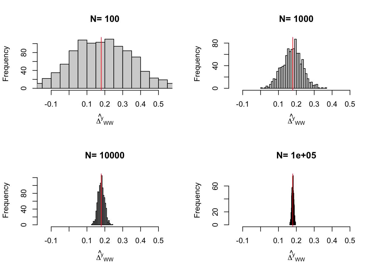
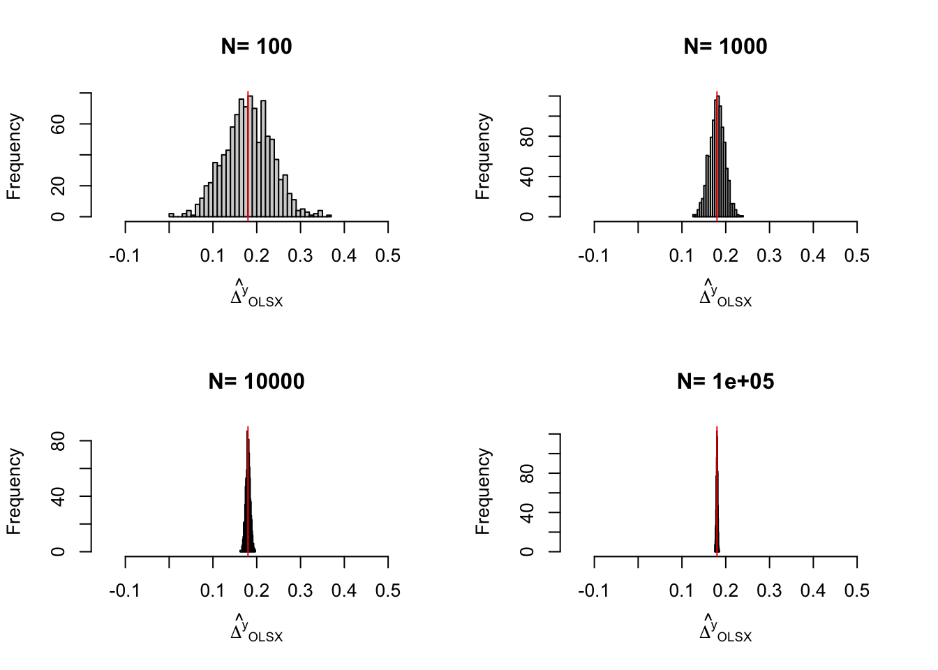
Figure 3.1: Distribution of the \(WW\) and \(OLSX\) estimators in a Brute Force design over replications of samples of different sizes
Figure 3.1 shows that the gains in precision from conditioning on \(y_i^B\) are spectacular in our numerical example. They basically correspond to a gain in one order of magnitude of sample size: the precision of the \(OLSX\) estimator conditioning on \(y_i^B\) with a sample size of 100 is similar to the precision of the \(OLS\) estimator not conditioning on \(y_i^B\) with a sample size of \(1000\). This large gain in precision is largely due to the fact that \(y_i\) and \(y_i^B\) are highly correlated. Not all covariates perform so well in actual samples in the social sciences.
Remark. The ability to condition on covariates in order to decrease sampling noise is a blessing but can also be a curse when combined with significance testing. Indeed, you can now see that you can run a lot of regressions (with and without some covariates, interactions, etc) and maybe report only the statistically significant ones. This is a bad practice that will lead to publication bias and inflated treatment effects. Several possibilities in order to avoid that:
- Pre-register your analysis and explain which covariates you are going to use (with which interactions, etc) so that you cannot cherry pick your favorite results ex-post.
- Use a stratified design for your RCT (more on this in Lecture 6) so that the important covariates are already balanced between treated and controls.
- If unable to do all of the above, report results from regressions without controls and with various sets of controls. We do not expect the various treatment effect estimates to be the same (they cannot be, otherwise, they would have similar sampling noise), but we expect the following pattern: conditioning should systematically decrease sampling noise, not increase the treatment effect estimate. If conditioning on covariates makes a treatment effect significant, pay attention to why: is it because of a decrease in sampling noise (expected and OK) or because of an increase in treatment effect (beware specification search).
Revise that especially in light of Chapter ??
Remark. You might not be happy with the assumption of linearity needed to use OLS to control for covariates. I have read somewhere (forgot where) that this should not be much of a problem since covariates are well balanced between groups by randomization, and thus a linear first approximation to the function relating \(X_i\) to \(Y_i\) should be fine. I tend not to buy that argument much. I have to run simulations with a non linear relation between outcomes and controls and see how linear OLS performs. If you do not like the linearity assumption, you can always use any of the nonparametric observational methods presented in Chapter ??.
3.1.3 Estimating Sampling Noise
In order to estimate sampling noise, you can either use the CLT-based approach or resampling, either using the bootstrap or randomization inference. In Section 2.2, we have already discussed how to estimate sampling noise when using the WW estimator that we are using here. We are going to use the default and heteroskedasticity-robust standard errors from OLS, which are both CLT-based. Only the heteroskedasticity-robust standard errors are valid under the assumptions that we have made so far. Homoskedasticity would require constant treatment effects. Heteroskedasticity being small in our numerical example, that should not matter much, but it could in other applications.
Example 3.7 Let us first estimate sampling noise for the simple WW estimator without control variables, using the OLS estimator.
sn.BF.simuls <- 2*quantile(abs(simuls.brute.force.ww[['1000']][,'WW']-delta.y.ate(param)),probs=c(0.99))
sn.BF.OLS.hetero <- 2*qnorm((delta+1)/2)*sqrt(vcovHC(reg.y.R.ols,type='HC2')[2,2])
sn.BF.OLS.homo <- 2*qnorm((delta+1)/2)*sqrt(vcov(reg.y.R.ols)[2,2])
The true value of the 99% sampling noise with a sample size of 1000 and no control variables is stemming from the simulations is 0.274. The 99% sampling noise estimated using heteroskedasticity robust OLS standard errors is 0.295. The 99% sampling noise estimated using default OLS standard errors is 0.294.
Let us now estimate sampling noise for the simple WW estimator conditioning on \(y_i^B\), using the OLS estimator.
sn.BF.simuls.yB <- 2*quantile(abs(simuls.brute.force.ww.yB[['1000']][,'WW']-delta.y.ate(param)),probs=c(0.99))
sn.BF.OLS.hetero.yB <- 2*qnorm((delta+1)/2)*sqrt(vcovHC(reg.y.R.ols.yB,type='HC2')[2,2])
sn.BF.OLS.homo.yB <- 2*qnorm((delta+1)/2)*sqrt(vcov(reg.y.R.ols.yB)[2,2])
The true value of the 99% sampling noise with a sample size of 1000 and with control variables stemming from the simulations is 0.088. The 99% sampling noise estimated using heteroskedasticity robust OLS standard errors is 0.092. The 99% sampling noise estimated using default OLS standard errors is 0.091.
Let’s see how all of this works on average. Figure 3.2 shows that overall the sampling nois eis much lower with \(OLSX\) than with \(WW\), as expected from Figure 3.1. The CLT-based estimator of sampling noise accounting for heteroskedasticity (in blue) recovers true sampling noise (in red) pretty well. Figure 3.3 shows that the CLT-based estimates of sampling noise are on point, except for \(N=10000\), where the CLT slightly overestimates true sampling noise. Figure 3.4 shows what happens when conditioning on \(Y^B\) in a selection of 40 samples. The reduction in samplong noise is pretty drastic here.
for (k in (1:length(N.sample))){
  simuls.brute.force.ww[[k]]$CLT.noise <- 2*qnorm((delta+1)/2)*simuls.brute.force.ww[[k]][,'se']
  simuls.brute.force.ww.yB[[k]]$CLT.noise <- 2*qnorm((delta+1)/2)*simuls.brute.force.ww.yB[[k]][,'se']
}

samp.noise.ww.BF <- sapply(lapply(simuls.brute.force.ww,`[`,,1),samp.noise,delta=delta)
precision.ww.BF <- sapply(lapply(simuls.brute.force.ww,`[`,,1),precision,delta=delta)
names(precision.ww.BF) <- N.sample
signal.to.noise.ww.BF <- sapply(lapply(simuls.brute.force.ww,`[`,,1),signal.to.noise,delta=delta,param=param)
names(signal.to.noise.ww.BF) <- N.sample
table.noise.BF <- cbind(samp.noise.ww.BF,precision.ww.BF,signal.to.noise.ww.BF)
colnames(table.noise.BF) <- c('sampling.noise', 'precision', 'signal.to.noise')
table.noise.BF <- as.data.frame(table.noise.BF)
table.noise.BF$N <- as.numeric(N.sample)
table.noise.BF$ATE <- rep(delta.y.ate(param),nrow(table.noise.BF))
for (k in (1:length(N.sample))){
  table.noise.BF$CLT.noise[k] <- mean(simuls.brute.force.ww[[k]]$CLT.noise)
}
table.noise.BF$Method <- rep("WW",nrow(table.noise.BF))

samp.noise.ww.BF.yB <- sapply(lapply(simuls.brute.force.ww.yB,`[`,,1),samp.noise,delta=delta)
precision.ww.BF.yB <- sapply(lapply(simuls.brute.force.ww.yB,`[`,,1),precision,delta=delta)
names(precision.ww.BF.yB) <- N.sample
signal.to.noise.ww.BF.yB <- sapply(lapply(simuls.brute.force.ww.yB,`[`,,1),signal.to.noise,delta=delta,param=param)
names(signal.to.noise.ww.BF.yB) <- N.sample
table.noise.BF.yB <- cbind(samp.noise.ww.BF.yB,precision.ww.BF.yB,signal.to.noise.ww.BF.yB)
colnames(table.noise.BF.yB) <- c('sampling.noise', 'precision', 'signal.to.noise')
table.noise.BF.yB <- as.data.frame(table.noise.BF.yB)
table.noise.BF.yB$N <- as.numeric(N.sample)
table.noise.BF.yB$ATE <- rep(delta.y.ate(param),nrow(table.noise.BF.yB))
for (k in (1:length(N.sample))){
  table.noise.BF.yB$CLT.noise[k] <- mean(simuls.brute.force.ww.yB[[k]]$CLT.noise)
}
table.noise.BF.yB$Method <- rep("OLSX",nrow(table.noise.BF))

table.noise.BF.tot <- rbind(table.noise.BF,table.noise.BF.yB)
table.noise.BF.tot$Method <- factor(table.noise.BF.tot$Method,levels=c("WW","OLSX"))

ggplot(table.noise.BF.tot, aes(x=as.factor(N), y=ATE,fill=Method)) +
  geom_bar(position=position_dodge(), stat="identity", colour='black') +
  geom_errorbar(aes(ymin=ATE-sampling.noise/2, ymax=ATE+sampling.noise/2), width=.2,position=position_dodge(.9),color='red') +
  geom_errorbar(aes(ymin=ATE-CLT.noise/2, ymax=ATE+CLT.noise/2), width=.2,position=position_dodge(.9),color='blue') +
  xlab("Sample Size")+
  theme_bw()+
  theme(legend.position=c(0.85,0.88))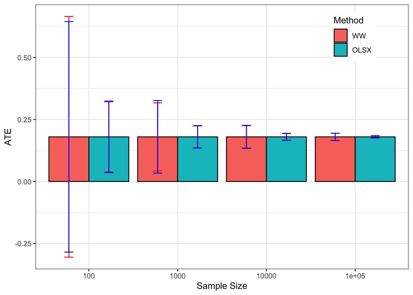
Figure 3.2: Average CLT-based approximations of sampling noise in the Brute Force design for \(WW\) and \(OLSX\) over replications of samples of different sizes (true sampling noise in red)
par(mfrow=c(2,2))
for (i in 1:length(simuls.brute.force.ww)){
  hist(simuls.brute.force.ww[[i]][,'CLT.noise'],main=paste('N=',as.character(N.sample[i])),xlab=expression(hat(2*bar(epsilon))[WW]),xlim=c(min(table.noise.BF[i,colnames(table.noise)=='sampling.noise'],min(simuls.brute.force.ww[[i]][,'CLT.noise'])),max(table.noise.BF[i,colnames(table.noise)=='sampling.noise'],max(simuls.brute.force.ww[[i]][,'CLT.noise']))))
  abline(v=table.noise.BF[i,colnames(table.noise)=='sampling.noise'],col="red")
}
par(mfrow=c(2,2))
for (i in 1:length(simuls.brute.force.ww.yB)){
  hist(simuls.brute.force.ww.yB[[i]][,'CLT.noise'],main=paste('N=',as.character(N.sample[i])),xlab=expression(hat(2*bar(epsilon))[OLSX]),xlim=c(min(table.noise.BF.yB[i,colnames(table.noise)=='sampling.noise'],min(simuls.brute.force.ww.yB[[i]][,'CLT.noise'])),max(table.noise.BF.yB[i,colnames(table.noise)=='sampling.noise'],max(simuls.brute.force.ww.yB[[i]][,'CLT.noise']))))
  abline(v=table.noise.BF.yB[i,colnames(table.noise)=='sampling.noise'],col="red")
}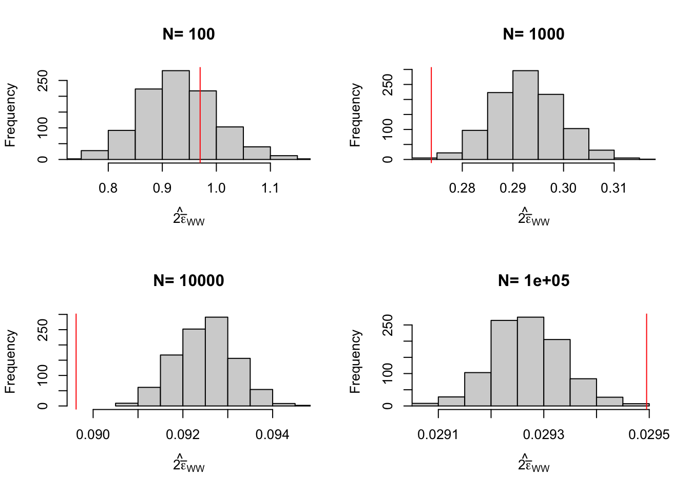
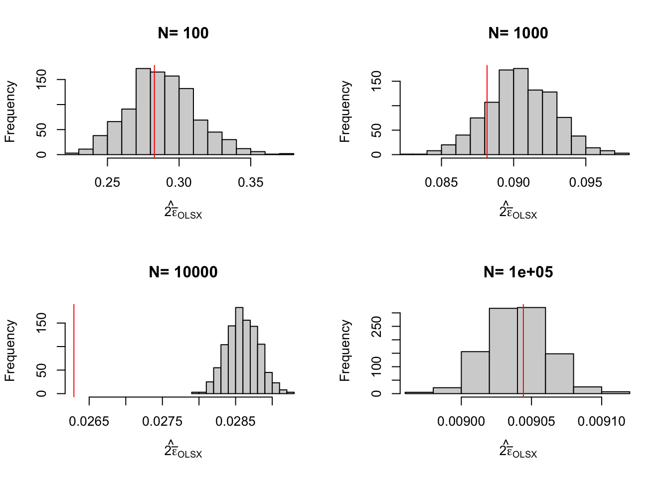
Figure 3.3: Distribution of the CLT approximation of sampling noise in the Brute Force design for \(WW\) and \(OLSX\) over replications of samples of different sizes (true sampling noise in red)
N.plot <- 40
plot.list <- list()
limx <- list(c(-0.65,1.25),c(-0.1,0.5),c(0,0.30),c(0,0.25))

for (k in 1:length(N.sample)){
  set.seed(1234)
  test.CLT.BF <- simuls.brute.force.ww[[k]][sample(N.plot),c('WW','CLT.noise')]
  test.CLT.BF <- as.data.frame(cbind(test.CLT.BF,rep(samp.noise(simuls.brute.force.ww[[k]][,'WW'],delta=delta),N.plot)))
  colnames(test.CLT.BF) <- c('WW','CLT.noise','sampling.noise')
  test.CLT.BF$id <- 1:N.plot
  plot.test.CLT.BF <- ggplot(test.CLT.BF, aes(x=as.factor(id), y=WW)) +
      geom_bar(position=position_dodge(), stat="identity", colour='black') +
      geom_errorbar(aes(ymin=WW-sampling.noise/2, ymax=WW+sampling.noise/2), width=.2,position=position_dodge(.9),color='red') +
      geom_errorbar(aes(ymin=WW-CLT.noise/2, ymax=WW+CLT.noise/2), width=.2,position=position_dodge(.9),color='blue') +
      geom_hline(aes(yintercept=delta.y.ate(param)), colour="#990000", linetype="dashed")+
      ylim(limx[[k]][1],limx[[k]][2])+
      xlab("Sample id")+
      theme_bw()+
      ggtitle(paste("N=",N.sample[k]))
  plot.list[[k]] <- plot.test.CLT.BF
}
plot.CI.BF <- plot_grid(plot.list[[1]],plot.list[[2]],plot.list[[3]],plot.list[[4]],ncol=1,nrow=length(N.sample))
print(plot.CI.BF)

plot.list <- list()
for (k in 1:length(N.sample)){
  set.seed(1234)
  test.CLT.BF.yB <- simuls.brute.force.ww.yB[[k]][sample(N.plot),c('WW','CLT.noise')]
  test.CLT.BF.yB <- as.data.frame(cbind(test.CLT.BF.yB,rep(samp.noise(simuls.brute.force.ww.yB[[k]][,'WW'],delta=delta),N.plot)))
  colnames(test.CLT.BF.yB) <- c('WW','CLT.noise','sampling.noise')
  test.CLT.BF.yB$id <- 1:N.plot
  plot.test.CLT.BF.yB <- ggplot(test.CLT.BF.yB, aes(x=as.factor(id), y=WW)) +
      geom_bar(position=position_dodge(), stat="identity", colour='black') +
      geom_errorbar(aes(ymin=WW-sampling.noise/2, ymax=WW+sampling.noise/2), width=.2,position=position_dodge(.9),color='red') +
      geom_errorbar(aes(ymin=WW-CLT.noise/2, ymax=WW+CLT.noise/2), width=.2,position=position_dodge(.9),color='blue') +
      geom_hline(aes(yintercept=delta.y.ate(param)), colour="#990000", linetype="dashed")+
      ylim(limx[[k]][1],limx[[k]][2])+
      xlab("Sample id")+
      ylab("OLSX")+
      theme_bw()+
      ggtitle(paste("N=",N.sample[k]))
  plot.list[[k]] <- plot.test.CLT.BF.yB
}
plot.CI.BF.yB <- plot_grid(plot.list[[1]],plot.list[[2]],plot.list[[3]],plot.list[[4]],ncol=1,nrow=length(N.sample))
print(plot.CI.BF.yB)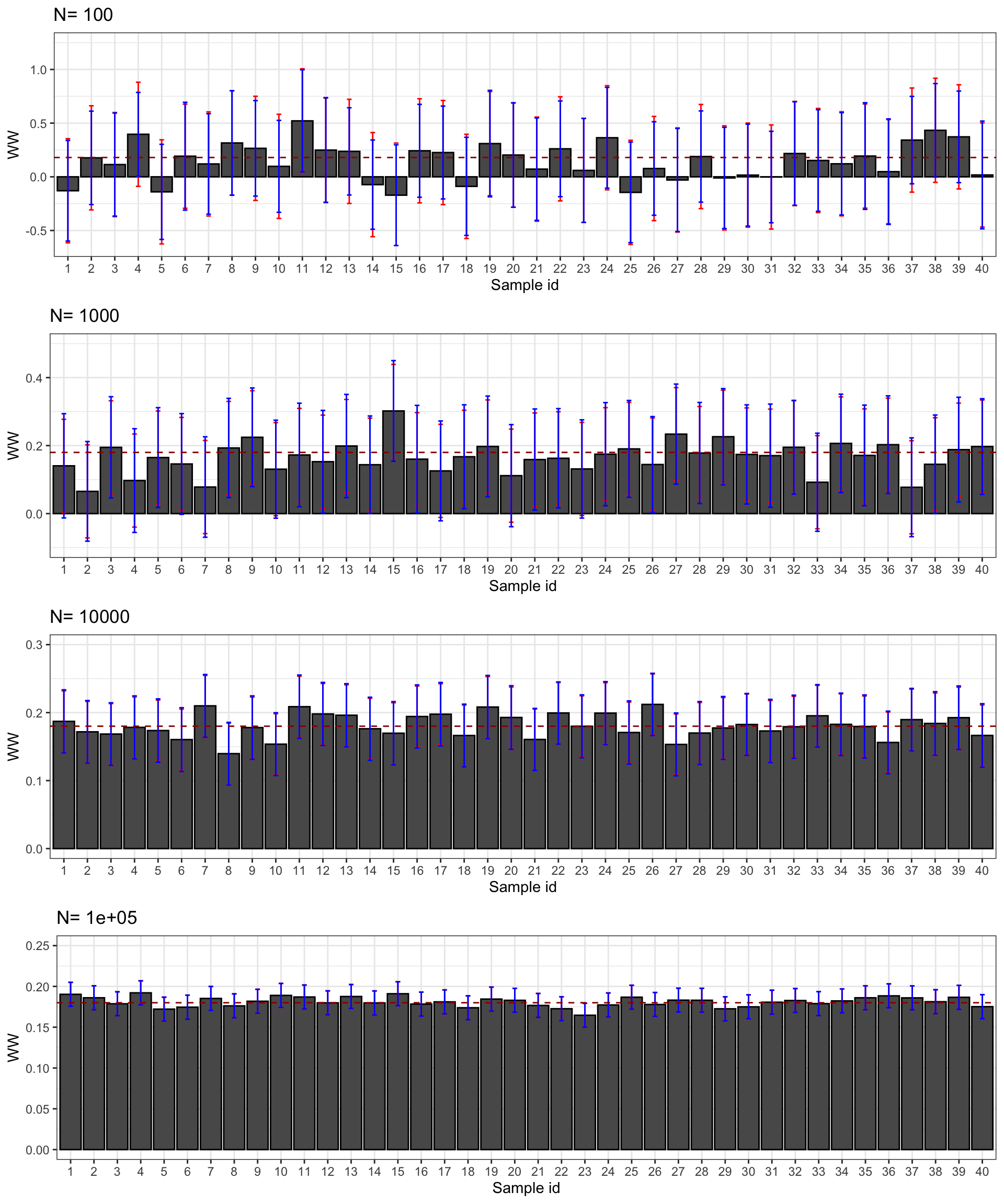
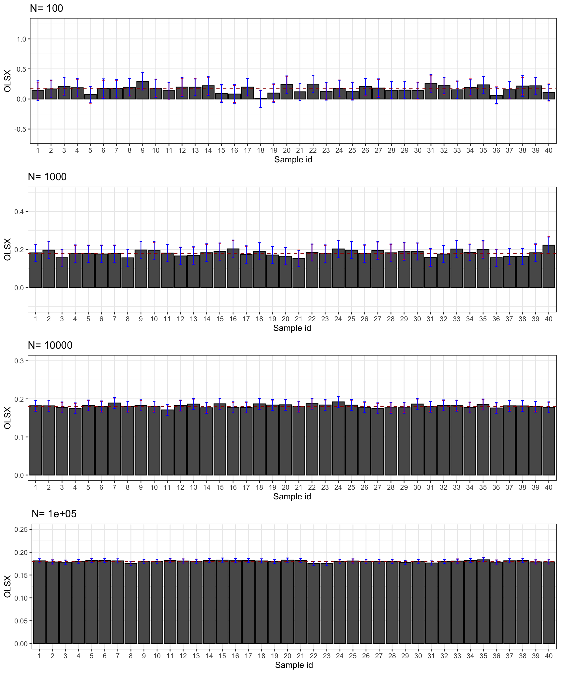
Figure 3.4: CLT-based confidence intervals of \(\hat{WW}\) and \(\hat{OLSX}\) for \(\delta=\) 0.99 over sample replications for various sample sizes (true confidence intervals in red)
3.2 Self-Selection design
In a Self-Selection design, individuals are randomly assigned to the treatment after having expressed their willingness to receive it. This design is able to recover the average effect of the Treatment on the Treated (TT).
In order to explain this design clearly, and especially to make it clear how it differs from the following one (randomization after eligibility), I have to introduce a slightly more complex selection rule that we have seen so far, one that includes self-selection, take-up decisions by agents. We are going to assume that there are two steps in agents’ participation process:
- Eligibility: agents’ eligibility is assessed first, giving rise to a group of eligible individuals (\(E_i=1\)) and a group of non eligible individuals (\(E_i=0\)).
- Self-selection: eligible agents can then decide whether they want to take-up the proposed treatment or not. \(D_i=1\) for those who do. \(D_i=0\) for those who do not. By convention, ineligibles have \(D_i=0\).
Example 3.8 In our numerical example, here are the equations operationalizing these notions:
\[\begin{align*} E_i & = \uns{y_i^B\leq\bar{y}} \\ D_i & = \uns{\underbrace{\bar{\alpha}+\theta\bar{\mu}-C_i}_{D_i^*}\geq0 \land E_i=1} \\ C_i & = \bar{c} + \gamma \mu_i + V_i\\ V_i & \sim \mathcal{N}(0,\sigma^2_V) \end{align*}\]
Eligibility is still decided based on pre-treatment outcomes being smaller than a threshold level \(\bar{y}\). Self-selection among eligibles is decided by the net utility of the treatment \(D_i^*\) being positive. Here, the net utility is composed of the average gain from the treatment (assuming agents cannot foresee their idiosyncratic gain from the treatment) \(\bar{\alpha}+\theta\bar{\mu}\) minus the cost of participation \(C_i\). The cost of participation in turn depends on a constant, on \(\mu_i\) and on a random shock orthogonal to everything else \(V_i\). This cost might represent the administrative cost of applying for the treatment and the opportunity cost of participating into the treatment (foregone earnings and/or cost of time). Conditional on eligiblity, self-selection is endogenous in this model since both the gains and the cost of participation depend on \(\mu_i\). Costs depend on \(\mu_i\) since most productive people may face lower administrative costs but a higher opportunity cost of time.
Let’s choose some values for the new parameters:
param <- c(param,-6.25,0.9,0.5)
names(param) <- c("barmu","sigma2mu","sigma2U","barY","rho","theta","sigma2epsilon","sigma2eta","delta","baralpha","barc","gamma","sigma2V")
and let’s generate a new dataset:
set.seed(1234)
N <-1000
mu <- rnorm(N,param["barmu"],sqrt(param["sigma2mu"]))
UB <- rnorm(N,0,sqrt(param["sigma2U"]))
yB <- mu + UB
YB <- exp(yB)
E <- ifelse(YB<=param["barY"],1,0)
V <- rnorm(N,0,param["sigma2V"])
Dstar <- param["baralpha"]+param["theta"]*param["barmu"]-param["barc"]-param["gamma"]*mu-V
Ds <- ifelse(Dstar>=0 & E==1,1,0)
epsilon <- rnorm(N,0,sqrt(param["sigma2epsilon"]))
eta<- rnorm(N,0,sqrt(param["sigma2eta"]))
U0 <- param["rho"]*UB + epsilon
y0 <- mu +  U0 + param["delta"]
alpha <- param["baralpha"]+  param["theta"]*mu + eta
y1 <- y0+alpha
Y0 <- exp(y0)
Y1 <- exp(y1)
Let’s compute the value of the TT parameter in this new model:
\[\begin{align*} \Delta^y_{TT} & = \bar{\alpha}+ \theta\esp{\mu_i|\mu_i+U_i^B\leq\bar{y} \land \bar{\alpha}+\theta\bar{\mu}-\bar{c}-\gamma\mu_i-V_i\geq0} \end{align*}\]
To compute the expectation of a doubly censored normal, I use the package tmvtnorm.
\[\begin{align*} (\mu_i,y_i^B,D_i^*) & = \mathcal{N}\left(\bar{\mu},\bar{\mu},\bar{\alpha}+(\theta-\gamma)\bar{\mu}-\bar{c}, \left(\begin{array}{ccc} \sigma^2_{\mu} & \sigma^2_{\mu} & -\gamma\sigma^2_{\mu} \\ \sigma^2_{\mu} & \sigma^2_{\mu} + \sigma^2_{U} & -\gamma\sigma^2_{\mu} \\ -\gamma\sigma^2_{\mu} & -\gamma\sigma^2_{\mu} & \gamma^2\sigma^2_{\mu}+\sigma^2_{V} \end{array} \right) \right) \end{align*}\]
mean.mu.yB.Dstar <- c(param['barmu'],param['barmu'],param['baralpha']- param['barc']+(param['theta']-param['gamma'])*param['barmu'])
cov.mu.yB.Dstar <- matrix(c(param['sigma2mu'],param["sigma2mu"],-param['gamma']*param["sigma2mu"],
                            param["sigma2mu"],param['sigma2mu']+param['sigma2U'],-param['gamma']*param["sigma2mu"],
                            -param['gamma']*param["sigma2mu"],-param['gamma']*param["sigma2mu"],param["sigma2mu"]*(param['gamma'])^2+param['sigma2V']),3,3,byrow=TRUE)
lower.cut <- c(-Inf,-Inf,0)
upper.cut <- c(Inf,log(param['barY']),Inf)
moments.cut <- mtmvnorm(mean=mean.mu.yB.Dstar,sigma=cov.mu.yB.Dstar,lower=lower.cut,upper=upper.cut)
delta.y.tt <- param['baralpha']+ param['theta']*moments.cut$tmean[1]
delta.y.ww.self.select <- mean(y[R==1 & Ds==1])-mean(y[R==0 & Ds==1])
The value of \(\Delta^y_{TT}\) in our illustration is now 0.17.
3.2.1 Identification
In a Self-Selection design, identification requires two assumptions:
Definition 3.3 (Independence Among Self-Selected) We assume that the randomized allocation of the program among applicants is well done:
\[\begin{align*} R_i\Ind(Y_i^0,Y_i^1)|D_i=1. \end{align*}\]
Independence can be enforced by the randomized allocation of the treatment among the eligible applicants.
We need a second assumption:
Definition 3.4 (Self-Selection design Validity) We assume that the randomized allocation of the program does not interfere with how potential outcomes and self-selection are generated:
\[\begin{align*} Y_i & = \begin{cases} Y_i^1 & \text{ if } (R_i=1 \text{ and } D_i=1) \\ Y_i^0 & \text{ if } (R_i=0 \text{ and } D_i=1) \text{ or } D_i=0 \end{cases} \end{align*}\]
with \(Y_i^1\), \(Y_i^0\) and \(D_i\) the same potential outcomes and self-selection decisions as in a routine allocation of the treatment.
Under these assumptions, we have the following result:
Theorem 3.2 (Identification in a Self-Selection design) Under Assumptions 3.3 and 3.4, the WW estimator among the self-selected identifies TT:
\[\begin{align*} \Delta^Y_{WW|D=1} & = \Delta^Y_{TT}, \end{align*}\]
with:
\[\begin{align*} \Delta^Y_{WW|D=1} & = \esp{Y_i|R_i=1,D_i=1} - \esp{Y_i|R_i=0,D_i=1}. \end{align*}\]
Proof. \[\begin{align*} \Delta^Y_{WW|D=1} & = \esp{Y_i|R_i=1,D_i=1} - \esp{Y_i|R_i=0,D_i=1} \\ & = \esp{Y^1_i|R_i=1,D_i=1} - \esp{Y^0_i|R_i=0,D_i=1} \\ & = \esp{Y_i^1|D_i=1}-\esp{Y_i^0|D_i=1}\\ & = \esp{Y_i^1-Y_i^0|D_i=1}, \end{align*}\] where the second equality uses Assummption3.4, the third equality Assumption 3.3 and the last equality the linearity of the expectation operator.
Remark. The key intuitions for how the Self-Selection design solves the FPCI are:
- By allowing for eligibilty and self-selection, we identify the agents that would benefit from the treatment in routine mode (the treated).
- By randomly denying the treatment to some of the treated, we can estimate the counterfactual outcome of the treated by looking at the counterfactual outcome of the denied applicants: \(\esp{Y_i^0|D_i=1}=\esp{Y_i|R_i=0,D_i=1}\).
Remark. In practice, we use a pseudo-RNG to generate a random allocation among applicants:
\[\begin{align*} R_i^* & \sim \mathcal{U}[0,1]\\ R_i & = \begin{cases} 1 & \text{ if } R_i^*\leq .5 \land D_i=1\\ 0 & \text{ if } R_i^*> .5 \land D_i=1 \end{cases} \end{align*}\]
Example 3.9 In our numerical example, the following R code generates two random groups, one treated and one control, and imposes the Assumption of Self-Selection design Validity:
3.2.2 Estimating TT
3.2.2.1 Using the WW Estimator
As in the case of the Brute Force Design, we can use the WW estimator to estimate the effect of the program with a Self-Selection design, except that this time the WW estimator is applied among applicants to the program only:
\[\begin{align*} \hat{\Delta}^Y_{WW|D=1} & = \frac{1}{\sum_{i=1}^N D_iR_i}\sum_{i=1}^N Y_iD_iR_i-\frac{1}{\sum_{i=1}^N D_i(1-R_i)}\sum_{i=1}^N D_iY_i(1-R_i). \end{align*}\]
Example 3.10 In our numerical example, we can form the WW estimator among applicants:
WW among applicants is equal to 0.085. It is actually rather far from the true value of 0.17, which reminds us that unbiasedness does not mean that a given sample will not suffer from a large bias. We just drew a bad sample where confounders are not very well balanced.
3.2.2.2 Using OLS
As in the Brute Force Design with the ATE, we can estimate the TT parameter with a Self-Selection design using the OLS estimator. In the following regression run among applicants only (with \(D_i=1\)), \(\beta\) estimates TT:
\[\begin{align*} Y_i & = \alpha + \beta R_i + U_i. \end{align*}\]
As a matter of fact, the OLS estimator without control variables is numerically equivalent to the WW estimator.
Example 3.11 In our numerical example, here is the OLS regression:
The value of the OLS estimator is 0.085, which is identical to the WW estimator among applicants.
3.2.2.3 Using OLS Conditioning on Covariates
We might want to condition on covariates in order to reduce the amount of sampling noise. Parametrically, we can run the following OLS regression among applicants (with \(D_i=1\)):
\[\begin{align*} Y_i & = \alpha + \beta R_i + \gamma' X_i + U_i. \end{align*}\]
\(\beta\) estimates the TT.
Needed: proof. Especially check whether we need to center covariates at the mean of the treatment group. I think so.
We can also use Matching to obtain a nonparametric estimator.
Example 3.12 Let us first compute the OLS estimator conditioning on \(y_i^B\):
Our estimate of TT after conditioning on \(y_i^B\) is 0.145. Conditioning on \(y_i^B\) has been able to solve part of the bias of the WW problem estimator.
Let’s now check whether conditioning on OLS has brought an improvement in terms of decreased sampling noise.
monte.carlo.self.select.ww <- function(s,N,param){
set.seed(s)
mu <- rnorm(N,param["barmu"],sqrt(param["sigma2mu"]))
UB <- rnorm(N,0,sqrt(param["sigma2U"]))
yB <- mu + UB
YB <- exp(yB)
E <- ifelse(YB<=param["barY"],1,0)
V <- rnorm(N,0,param["sigma2V"])
Dstar <- param["baralpha"]+param["theta"]*param["barmu"]-param["barc"]-param["gamma"]*mu-V
Ds <- ifelse(Dstar>=0 & E==1,1,0)
epsilon <- rnorm(N,0,sqrt(param["sigma2epsilon"]))
eta<- rnorm(N,0,sqrt(param["sigma2eta"]))
U0 <- param["rho"]*UB + epsilon
y0 <- mu + U0 + param["delta"]
alpha <- param["baralpha"]+ param["theta"]*mu + eta
y1 <- y0+alpha
Y0 <- exp(y0)
Y1 <- exp(y1)
#random allocation among self-selected
Rs <- runif(N)
R <- ifelse(Rs<=.5 & Ds==1,1,0)
y <- y1*R+y0*(1-R)
Y <- Y1*R+Y0*(1-R)
return(mean(y[R==1 & Ds==1])-mean(y[R==0 & Ds==1]))
}
simuls.self.select.ww.N <- function(N,Nsim,param){
simuls.self.select.ww <- matrix(unlist(lapply(1:Nsim,monte.carlo.self.select.ww,N=N,param=param)),nrow=Nsim,ncol=1,byrow=TRUE)
colnames(simuls.self.select.ww) <- c('WW')
return(simuls.self.select.ww)
}
sf.simuls.self.select.ww.N <- function(N,Nsim,param){
sfInit(parallel=TRUE,cpus=8)
sim <- matrix(unlist(sfLapply(1:Nsim,monte.carlo.self.select.ww,N=N,param=param)),nrow=Nsim,ncol=1,byrow=TRUE)
sfStop()
colnames(sim) <- c('WW')
return(sim)
}
Nsim <- 1000
#Nsim <- 10
N.sample <- c(100,1000,10000,100000)
#N.sample <- c(100,1000,10000)
#N.sample <- c(100,1000)
#N.sample <- c(100)
simuls.self.select.ww <- lapply(N.sample,sf.simuls.self.select.ww.N,Nsim=Nsim,param=param)
names(simuls.self.select.ww) <- N.samplemonte.carlo.self.select.yB.ww <- function(s,N,param){
set.seed(s)
mu <- rnorm(N,param["barmu"],sqrt(param["sigma2mu"]))
UB <- rnorm(N,0,sqrt(param["sigma2U"]))
yB <- mu + UB
YB <- exp(yB)
E <- ifelse(YB<=param["barY"],1,0)
V <- rnorm(N,0,param["sigma2V"])
Dstar <- param["baralpha"]+param["theta"]*param["barmu"]-param["barc"]-param["gamma"]*mu-V
Ds <- ifelse(Dstar>=0 & E==1,1,0)
epsilon <- rnorm(N,0,sqrt(param["sigma2epsilon"]))
eta<- rnorm(N,0,sqrt(param["sigma2eta"]))
U0 <- param["rho"]*UB + epsilon
y0 <- mu + U0 + param["delta"]
alpha <- param["baralpha"]+ param["theta"]*mu + eta
y1 <- y0+alpha
Y0 <- exp(y0)
Y1 <- exp(y1)
#random allocation among self-selected
Rs <- runif(N)
R <- ifelse(Rs<=.5 & Ds==1,1,0)
y <- y1*R+y0*(1-R)
Y <- Y1*R+Y0*(1-R)
reg.y.R.yB.ols.self.select <- lm(y[Ds==1] ~ R[Ds==1] + yB[Ds==1])
return(reg.y.R.yB.ols.self.select$coef[2])
}
simuls.self.select.yB.ww.N <- function(N,Nsim,param){
simuls.self.select.yB.ww <- matrix(unlist(lapply(1:Nsim,monte.carlo.self.select.yB.ww,N=N,param=param)),nrow=Nsim,ncol=1,byrow=TRUE)
colnames(simuls.self.select.yB.ww) <- c('WW')
return(simuls.self.select.yB.ww)
}
sf.simuls.self.select.yB.ww.N <- function(N,Nsim,param){
sfInit(parallel=TRUE,cpus=8)
sim <- matrix(unlist(sfLapply(1:Nsim,monte.carlo.self.select.yB.ww,N=N,param=param)),nrow=Nsim,ncol=1,byrow=TRUE)
sfStop()
colnames(sim) <- c('WW')
return(sim)
}
Nsim <- 1000
#Nsim <- 10
N.sample <- c(100,1000,10000,100000)
#N.sample <- c(100,1000,10000)
#N.sample <- c(100,1000)
#N.sample <- c(100)
simuls.self.select.yB.ww <- lapply(N.sample,sf.simuls.self.select.yB.ww.N,Nsim=Nsim,param=param)
names(simuls.self.select.yB.ww) <- N.samplepar(mfrow=c(2,2))
for (i in 1:length(simuls.self.select.ww)){
hist(simuls.self.select.ww[[i]][,'WW'],breaks=30,main=paste('N=',as.character(N.sample[i])),xlab=expression(hat(Delta^yWW)),xlim=c(-0.15,0.55))
abline(v=delta.y.tt,col="red")
}
par(mfrow=c(2,2))
for (i in 1:length(simuls.self.select.yB.ww)){
hist(simuls.self.select.yB.ww[[i]][,'WW'],breaks=30,main=paste('N=',as.character(N.sample[i])),xlab=expression(hat(Delta^yWW)),xlim=c(-0.15,0.55))
abline(v=delta.y.tt,col="red")
}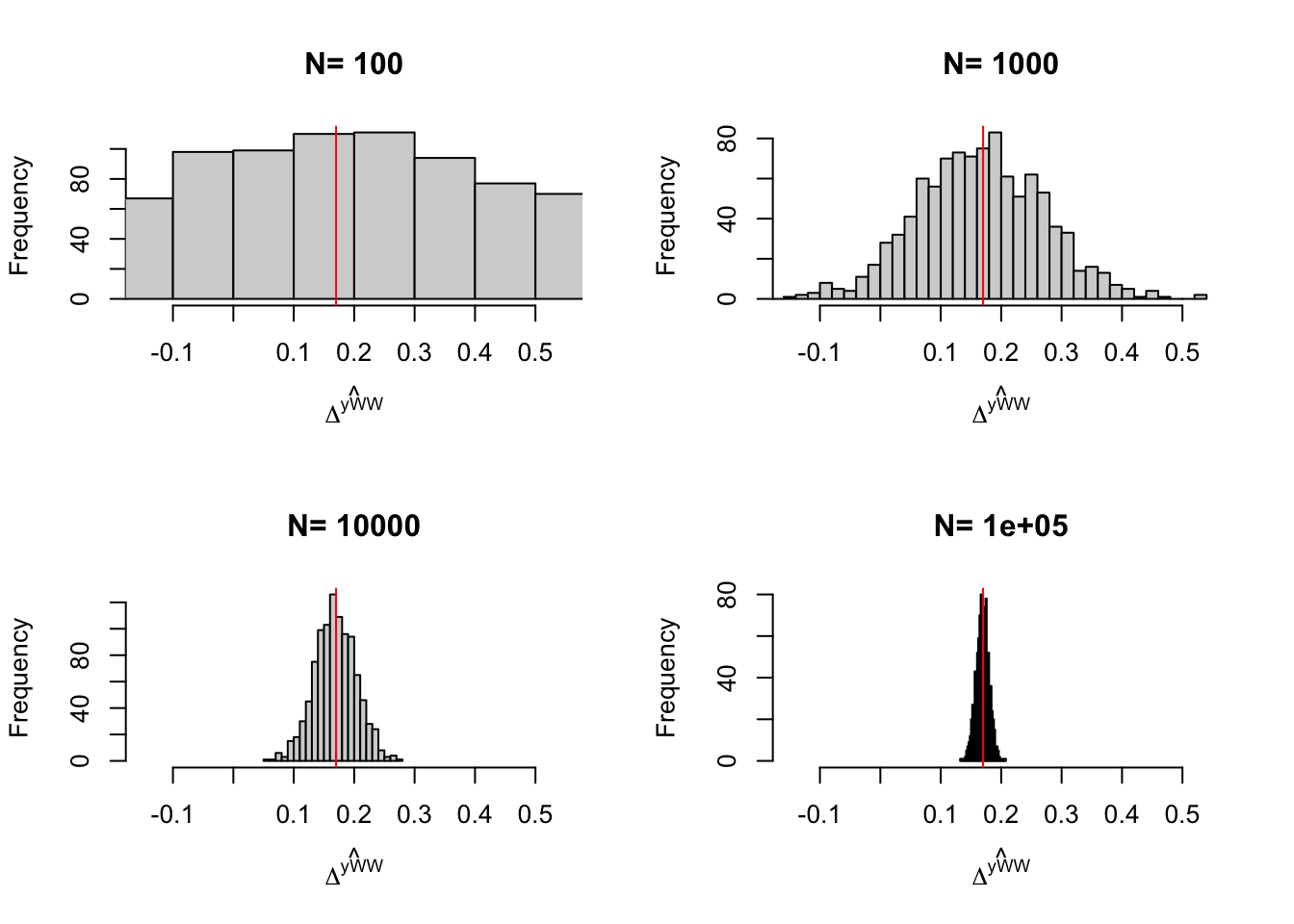
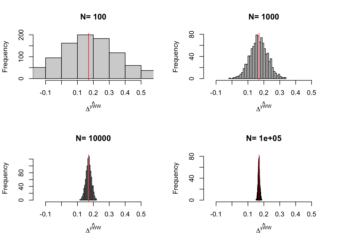
Figure 3.5: Distribution of the \(WW\) and \(OLSX\) estimator in a Self-Selection design over replications of samples of different sizes
Figure 3.5 shows that, in our example, conditioning on covariates improves precision by the same amount as an increase in sample size by almost one order of magnitude.
3.2.3 Estimating Sampling Noise
In order to estimate precision, we can either use the CLT, deriving sampling noise from the heteroskedasticity-robust standard error OLS estimates, or we can use some form of resampling as the bootstrap or randomization inference.
Example 3.13 Let us derive the CLT-based estimates of sampling noise using the OLS standard errors without conditioning on covariates first. I’m using the sample size with \(N=1000\) as an example.
sn.RASS.simuls <- 2*quantile(abs(simuls.self.select.ww[['1000']][,'WW']-delta.y.tt),probs=c(0.99))
sn.RASS.OLS.homo <- 2*qnorm((.99+1)/2)*sqrt(vcov(reg.y.R.ols.self.select)[2,2])
sn.RASS.OLS.hetero <- 2*qnorm((.99+1)/2)*sqrt(vcovHC(reg.y.R.ols.self.select,type='HC2')[2,2])
True 99% sampling noise (from the simulations) is 0.548. 99% sampling noise estimated using default OLS standard errors is 0.578. 99% sampling noise estimated using heteroskedasticity robust OLS standard errors is 0.58.
Conditioning on covariates:
sn.RASS.simuls.yB <- 2*quantile(abs(simuls.self.select.yB.ww[['1000']][,'WW']-delta.y.tt),probs=c(0.99))
sn.RASS.OLS.homo.yB <- 2*qnorm((.99+1)/2)*sqrt(vcov(reg.y.R.yB.ols.self.select)[2,2])
sn.RASS.OLS.hetero.yB <- 2*qnorm((.99+1)/2)*sqrt(vcovHC(reg.y.R.yB.ols.self.select,type='HC2')[2,2])
True 99% sampling noise (from the simulations) is 0.295. 99% sampling noise estimated using default OLS standard errors is 0.294. 99% sampling noise estimated using heteroskedasticity robust OLS standard errors is 0.299.
3.3 Eligibility design
In an Eligibility design, we randomly select two groups among the eligibles. Members of the treated group are informed that they are eligible to the program and are free to self-select into it. Members of the control group are not enformed that they are eligible and cannot enroll into the program. In an Eligibility design, we can still recover the TT despite the fact that we have not randomized access to the programs among the applicants. This is the magic of instrumental variables. Let us detail the mechanics of this beautiful result.
3.3.1 Identification
In order to state the identification results in the Randomization After Eligibility design rigorously, I need to define new potential outcomes:
- \(Y_i^{d,r}\) is the value of the outcome \(Y\) when individual \(i\) belongs to the program group \(d\) (\(d\in\left\{0,1\right\}\)) and has been randomized in group \(r\) (\(r\in\left\{0,1\right\}\)).
- \(D_i^r\) is the value of the program participation decision when individual \(i\) has been assigned randomly to group \(r\).
3.3.1.1 Identification of TT
In an Eligiblity design, we need three assumptions to ensure identification of the TT:
Definition 3.5 (Independence Among Eligibles) We assume that the randomized allocation of the program among eligibles is well done:
\[\begin{align*} R_i\Ind(Y_i^{0,0},Y_i^{0,1},Y_i^{1,0},Y_i^{1,1},D_i^1,D_i^0)|E_i=1. \end{align*}\]
Independence can be enforced by the randomized allocation of information about eligibility among the eligibles.
We need a second assumption:
Definition 3.6 (Randomization After Eligibility Validity) We assume that no eligibles that has been randomized out can take the treatment and that the randomized allocation of the program does not interfere with how potential outcomes and self-selection are generated:
\[\begin{align*} D_i^0 & = 0\text{, } \forall i, \\ D_i & = D_i^1R_i+(1-R_i)D_i^0 \\ Y_i & = \begin{cases} Y_i^{1,1} & \text{ if } (R_i=1 \text{ and } D_i=1) \\ Y_i^{0,1} & \text{ if } (R_i=1 \text{ and } D_i=0) \\ Y_i^{0,0} & \text{ if } R_i=0 \end{cases} \end{align*}\]
with \(Y_i^{1,1}\), \(Y_i^{0,1}\), \(Y_i^{0,0}\), \(D_i^1\) and \(D^0_i\) the same potential outcomes and self-selection decisions as in a routine allocation of the treatment.
We need a third assumption:
Definition 3.7 (Exclusion Restriction of Eligibility) We assume that there is no direct effect of being informed about eligibliity to the program on outcomes:
\[\begin{align*} Y_i^{1,1} & = Y_i^{1,0}= Y_i^1\\ Y_i^{0,1} & = Y_i^{0,0}= Y_i^0. \end{align*}\]
Under these assumptions, we have the following result:
Theorem 3.3 (Identification of TT With Randomization After Eligibility) Under Assumptions 3.5, 3.6 and 3.7, the Bloom estimator among eligibles identifies TT:
\[\begin{align*} \Delta^Y_{Bloom|E=1} & = \Delta^Y_{TT}, \end{align*}\]
with:
\[\begin{align*} \Delta^Y_{Bloom|E=1} & = \frac{\Delta^Y_{WW|E=1}}{\Pr(D_i=1|R_i=1,E_i=1)} \\ \Delta^Y_{WW|E=1} & =\esp{Y_i|R_i=1,E_i=1}-\esp{Y_i|R_i=0,E_i=1}. \end{align*}\]
Proof. I keep the conditioning on \(E_i=1\) implicit all along to save notation.
\[\begin{align*} \esp{Y_i|R_i=1} & = \esp{Y_i^{1,1}D_i+Y_i^{0,1}(1-D_i)|R_i=1} \\ & = \esp{Y_i^0+D_i(Y_i^1-Y_i^0)|R_i=1} \\ & = \esp{Y_i^0|R_i=1}+\esp{Y_i^1-Y_i^0|D_i=1,R_i=1}\Pr(D_i=1|R_i=1)\\ & = \esp{Y_i^0}+\esp{Y_i^1-Y_i^0|D_i=1}\Pr(D_i=1|R_i=1), \end{align*}\]
where the first equality uses Assumption 3.6, the second equality Assumption 3.7 and the last equality Assumption 3.5 and the fact that \(D_i=1\Rightarrow R_i=1\). Using the same reasoning, we also have:
\[\begin{align*} \esp{Y_i|R_i=0} & = \esp{Y_i^{1,0}D_i+Y_i^{0,0}(1-D_i)|R_i=0} \\ & = \esp{Y_i^0|R_i=0} \\ & = \esp{Y_i^0}. \end{align*}\]
A direct application of the formula for the Bloom estimator proves the result.
3.3.1.2 Identification of ITE
The previous proof does not give a lot of intuition of how TT is identified in the Randomization After Eligibility design. In order to gain more insight, we are going to decompose the Bloom estimator, and have a look at its numerator. The numerator of the Bloom estimator is a With/Without comparison, and it identifies, under fairly light conditions, another causal effect, the Intention to Treat Effect (ITE).
Let me first define the ITE:
Definition 3.8 (Intention to Treat Effect) In a Randomization After Eligibility design, the Intention to Treat Effect (ITE) is the effect of receiving information about eligiblity among eligibles:
\[\begin{align*} \Delta^Y_{ITE} & = \esp{Y_i^{D_i^1,1}-Y_i^{D_i^0,0}|E_i=1}. \end{align*}\]
Receiving information about eligibility has two impacts, in the general framework that we have delineated so far: first, it triggers some individuals into the treatment (those for which \(D_i^1\neq0\)); second, it might have a direct effect on outcomes (\(Y_i^{d,1}\neq Y_i^{d,0}\)). This second effect is the effect of annoucing eligiblity that does not goes through participation into the program. For example, it is possible that announcing eligibility to a retirement program makes me save more for retirement, even if I end up not taking up the proposed program.
The two causal channels that are at work within the ITE can be seen more clearly after some manipulations:
\[\begin{align} \Delta^Y_{ITE} & = \esp{Y_i^{1,1}D^1_i+Y_i^{0,1}(1-D_i^1)-(Y_i^{1,0}D^0_i+Y_i^{0,0}(1-D_i^0))|E_i=1}\nonumber \\ & = \esp{Y_i^{1,1}D^1_i+Y_i^{0,1}(1-D_i^1)-(Y_i^{0,0}(D_i^1+1-D_i^1))|E_i=1}\nonumber \\ & = \esp{(Y_i^{1,1}-Y_i^{0,0})D^1_i+(Y_i^{0,1}-Y_i^{0,0})(1-D_i^1)|E_i=1}\nonumber \\ & = \esp{Y_i^{1,1}-Y_i^{0,0}|D^1_i=1,E_i=1}\Pr(D^1_i=1|E_i=1)\nonumber \\ & \phantom{=}+\esp{Y_i^{0,1}-Y_i^{0,0}|D_i^1=0,E_i=1}\Pr(D_i^1=0|E_i=1),\tag{3.1} \end{align}\]
where the first equality follows from Assumption 3.6 and the second equality uses the fact that \(D_i^0=0\), \(\forall i\).
We can now see that the ITE is composed of two terms: the first term captures the effect of announcing eligibility on those who decide to participate into the program; the second term captures the effect of announcing eligibility on those who do not participate into the program. Both of these effects are weighted by the respective proportions of those reacting to the eligibility annoucement by participating and by not participating respectively.
Now, in order to see how the ITE “contains” the TT, we can use the following theorem:
Theorem 3.4 (From ITE to TT) Under Assumptions 3.5, 3.6 and 3.7, ITE is equal to TT multiplied by the proportion of individuals taking up the treatment after eligibility has been announced:
\[\begin{align*} \Delta^Y_{ITE} & = \Delta^Y_{TT}\Pr(D^1_i=1|E_i=1). \end{align*}\]
Proof. Under Assumption 3.7, Equation (3.1) becomes:
\[\begin{align*} \Delta^Y_{ITE} & = \esp{Y_i^{1}-Y_i^{0}|D^1_i=1,E_i=1}\Pr(D^1_i=1|E_i=1) \\ & \phantom{=}+\esp{Y_i^{0}-Y_i^{0}|D_i^1=0,E_i=1}\Pr(D_i^1=0|E_i=1)\\ & = \esp{D_i^1(Y_i^{1}-Y_i^{0})|R_i=1,E_i=1} \\ & = \esp{Y_i^{1}-Y_i^{0}|D_i^1=1,R_i=1,E_i=1}\Pr(D^1_i=1|R_i=1,E_i=1) \\ & = \esp{Y_i^{1}-Y_i^{0}|D_i=1,E_i=1}\Pr(D^1_i=1|E_i=1), \end{align*}\]
where the first equality follows from Assumption 3.7, the second from Bayes’ rule and Assumptions 3.5, the third from Bayes’ rule and the last from the fact that \(D_i^1=1,R_i=1\Leftrightarrow D_i=1\).
The previous theorem shows that Assumption 3.7 shuts down any direct effect of the announcement of eligibility on outcomes. As a consequence of this assumption, the only impact that an eligibility annoucement has on outcomes is through participation into the program. Hence, the ITE is equal to TT multiplied by the proportion of people taking up the treatment when eligibility is announced.
In order to move from the link between TT and ITE to the mechanics of the Bloom estimator, we need two additional identification results. The first result shows that ITE can be identified under fairly light conditions by a WW estimator. The second result shows that the proportion of people taking up the treatment when eligiblity is announced is also easily estimated from the data.
Theorem 3.5 (Identification of ITE with Randomization After Eligibility) Under Assumptions 3.5 and 3.6, ITE is identified by the With/Without comparison among eligibles:
\[\begin{align*} \Delta^Y_{ITE} & = \Delta^Y_{WW|E=1}. \end{align*}\]
Proof. \[\begin{align*} \Delta^Y_{WW|E=1} & =\esp{Y_i|R_i=1,E_i=1}-\esp{Y_i|R_i=0,E_i=1} \\ & = \esp{Y_i^{D_i^1,1}|R_i=1,E_i=1}-\esp{Y_i^{D_i^0,0}|R_i=0,E_i=1} \\ & = \esp{Y_i^{D_i^1,1}|E_i=1}-\esp{Y_i^{D_i^0,0}|E_i=1}, \end{align*}\] where the second equality follows from Assumption 3.6 and the third from Assumption 3.5.
Theorem 3.6 (Identification of $\Pr(D^1_i=1|E_i=1)$) Under Assumptions 3.5 and 3.6, \(\Pr(D^1_i=1|E_i=1)\) is identified by the proportion of people taking up the offered treatment when informed about their eligibility status:
\[\begin{align*} \Pr(D^1_i=1|E_i=1) & = \Pr(D_i=1|R_i=1,E_i=1). \end{align*}\]
Proof. \[\begin{align*} \Pr(D_i=1|R_i=1,E_i=1) & =\Pr(D^1_i=1|R_i=1,E_i=1) \\ & = \Pr(D^1_i=1|E_i=1), \end{align*}\]
where the first equality follows from Assumption 3.6 and the second from Assumption 3.5.
Corollary 3.1 (Bloom estimator and ITE) It follows from Theorems 3.5 and 3.6 that, under Assumptions 3.5 and 3.6, the Bloom estimator is equal to the ITE divided by the propotion of agents taking up the program when eligible:
\[\begin{align*} \Delta^Y_{Bloom|E=1} & = \frac{\Delta^Y_{ITE}}{\Pr(D^1_i=1|E_i=1)}. \end{align*}\]
As a consequence of Corollary 3.1, we see that the Bloom estimator reweights the ITE, the effect of receiving information about eligibility, by the proportion of people reacting to the eligibility by participating in the program. From Theorem 3.4, we know that this ratio will be equal to TT if the Assumption 3.7 also holds, so that all the impact of the eligibility annoucement stems from entering the program. The eligibility annoucement serves as an instrument for program participation.
Remark. The design using Randomization After Eligibility seems like magic. You do not assign randomly the program, but information about the eligiblity status, but you can recover the effect of the program anyway. How does this magic work? Randomization After Eligibility is also less intrusive than Self-Selection design. With the latter design, you have to actively send away individuals that have expressed an interest for entering the program. This is harsh. With Randomization After Eligibility, you do not have to send away people expressing interest after being informed. And it seems that you are not paying a price for that, since you are able to recover the same TT parameter. Well, actually, you are going to pay a price in terms of larger sampling noise.
The intuition for all that can be delineated using the very same apparatus that we have developed so far. So here goes. Under the assumptions made so far, it is easy to show that (omitting the conditioning on \(E_i=1\) for simplicity):
\[\begin{align*} \Delta^Y_{WW|E=1} & = \esp{Y_i^{1,1}|D_i^1=1,R_i=1}\Pr(D^1_i=1|R_i=1)\\ & \phantom{=}-\esp{Y_i^{0,0}|D_i^1=1,R_i=0}\Pr(D^1_i=1|R_i=0) \\ & \phantom{=}+ \esp{Y_i^{0,1}|D_i^1=0,R_i=1}\Pr(D^1_i=0|R_i=1)\\ & \phantom{=}-\esp{Y_i^{0,0}|D_i^1=0,R_i=0}\Pr(D^1_i=0|R_i=0). \end{align*}\]
The first part of the equation is due to the difference in outcomes between the two treatment arms for people that take up the program when eligibility is announced. The second part is due to the difference in outcomes between the two treatment arms for people that do not take up the program when eligibility is announced. This second part cancels out under Assumption 3.5 and 3.7.
But this cancelling out only happens in the population. In a given sample, the sample equivalents to the two members of the second part of the equation do not have to be equal, and thus they do not cancel out, generating additional sampling noise compared to the Self-Selection design. Indeed, in the Self-Selection design, you observe the population with \(D_i^1=1\) in both the treatment and control arms (you actually observe this population before randomizing the treatment within it), and you can enforce that the effect on \(D_i^1=0\) should be zero, under your assumptions. In an Eligibility design, you do not observe the population with \(D_i^1=1\) in the control arm, and you cannot enforce the equality of the outcomes for those with \(D_i^1=0\) present in both arms. You have to rely on the sampling estimates to make this cancellation, and that generates sampling noise.
Remark. In practice, we use a pseudo-RNG to allocate the randomized annoucement of the eligibility status:
\[\begin{align*} R_i^* & \sim \mathcal{U}[0,1]\\ R_i & = \begin{cases} 1 & \text{ if } R_i^*\leq .5 \land E_i=1\\ 0 & \text{ if } R_i^*> .5 \land E_i=1 \end{cases} \\ D_i & = \uns{\bar{\alpha}+\theta\bar{\mu}-C_i\geq0 \land E_i=1 \land R_i=1} \end{align*}\]
Example 3.14 In our numerical example, we can actually use the same sample as we did for Self-Selection design. I have to generate it again, though, since I am going to allocate \(R_i\) differently.
set.seed(1234)
N <-1000
mu <- rnorm(N,param["barmu"],sqrt(param["sigma2mu"]))
UB <- rnorm(N,0,sqrt(param["sigma2U"]))
yB <- mu + UB
YB <- exp(yB)
E <- ifelse(YB<=param["barY"],1,0)
V <- rnorm(N,0,param["sigma2V"])
Dindex <- param["baralpha"]+param["theta"]*param["barmu"]-param["barc"]-param["gamma"]*mu-V
Dstar <- ifelse(Dindex>=0 & E==1,1,0)
epsilon <- rnorm(N,0,sqrt(param["sigma2epsilon"]))
eta<- rnorm(N,0,sqrt(param["sigma2eta"]))
U0 <- param["rho"]*UB + epsilon
y0 <- mu +  U0 + param["delta"]
alpha <- param["baralpha"]+  param["theta"]*mu + eta
y1 <- y0+alpha
Y0 <- exp(y0)
Y1 <- exp(y1)
The value of TT in our example is the same as the one in the Self-Selection design case. TT in the population is equal to 0.17.
Let’s now compute the value of ITE in the population. In our model, exclusion restriction holds, so that we can use the fact that \(ITE=TT\Pr(D^1_i=1|E_i=1)\). We thus only need to compute \(\Pr(D^1_i=1|E_i=1)\):
\[\begin{align*} \Pr(D^1_i=1|E_i=1) & = \Pr(D_i^*\geq0|y_i^B\leq\bar{y}). \end{align*}\]
I can again use the package tmvtnorm to compute that probability.
It is indeed equal to \(1-\Pr(D_i^*<0|y_i^B\leq\bar{y})\), where \(\Pr(D_i^*<0|y_i^B\leq\bar{y})\) is the cumulative density of \(D_i^*\) conditional on \(y_i^B\leq\bar{y}\), the marginal cumulative of the third variable of the truncated trivariate normal \((\mu_i,y_i^B,D_i^*)\) where the first variable is not truncated and the second one is truncated at \(\bar{y}\).
lower.cut <- c(-Inf,-Inf,-Inf)
upper.cut <- c(Inf,log(param['barY']),Inf)
prD1.elig <- 1-ptmvnorm.marginal(xn=0,n=3,mean=mean.mu.yB.Dstar,sigma=cov.mu.yB.Dstar,lower=lower.cut,upper=upper.cut)
delta.y.ite <- delta.y.tt*prD1.elig
\(\Pr(D^1_i=1|E_i=1)=\) 0.459. As a consequence, ITE in the population is equal to 0.17 * 0.459 \(\approx\) 0.078. In the sample, the value of ITE and TT are equal to:
delta.y.tt.sample <- mean(y1[E==1 & Dstar==1]-y0[E==1 & Dstar==1])
delta.y.ite.sample <- delta.y.tt.sample*mean(Dstar[E==1])
\(\Delta^y_{ITE_s}=\) 0.068 and \(\Delta^y_{TT_s}=\) 0.187.
Now, we can allocate the randomized treatment and let potential outcomes be realized:
3.3.2 Estimating the ITE and the TT
In general, we start the analysis of an Eligibility design by estimating the ITE. Then, we provide the TT by dividing the ITE by the proportion of participants among the eligibles.
Actually, this procedure is akin to an instrumental variables estimator and we will see that the Bloom estimator is actually an IV estimator. The ITE estimation step corresponds to the reduced form in a classical IV approach. Estimation of the proportion of participants is the first stage in a IV approach. Estimation of the TT corresponds to the structural equation step of an IV procedure.
3.3.2.1 Estimating the ITE
Estimation of the ITE relies on the WW estimator, in general implemented using OLS. It is similar to the estimation of ATE and TT in the Brute Force and Self-Selection designs.
3.3.2.1.1 Using the WW estimator
Estimation of the ITE can be based on the WW estimator among eligibles.
\[\begin{align*} \hat{\Delta}^Y_{WW|E=1} & = \frac{1}{\sum_{i=1}^N E_iR_i}\sum_{i=1}^N Y_iE_iR_i-\frac{1}{\sum_{i=1}^N E_i(1-R_i)}\sum_{i=1}^N E_iY_i(1-R_i). \end{align*}\]
Example 3.15 In our numerical example, we can form the WW estimator among eligibles:
WW among eligibles is equal to 0.069.
3.3.2.1.2 Using OLS
As we have already seen before, the WW estimator is equivalent to OLS with one constant and no control variables. As a consequence, we can estimate the ITE using the OLS estimate of \(\beta\) in the following regression run on the sample with \(E_i=1\):
\[\begin{align*} Y_i & = \alpha + \beta R_i + U_i. \end{align*}\]
By construction, \(\hat{\beta}_{OLSR|E=1}=\hat{\Delta}^Y_{WW|E=1}\).
Example 3.16 In our numerical example, we can form the WW estimator among eligibles:
\(\hat{\beta}_{OLSR|E=1}\) is equal to 0.069. Remember that ITE in the population is equal to 0.078.
3.3.2.1.3 Using OLS conditioning on covariates
Again, as in the previous designs, we can compute ITE by using OLS conditional on covariates. Parametrically, we can run the following OLS regression among eligibles (with \(E_i=1\)):
\[\begin{align*} Y_i & = \alpha + \beta R_i + \gamma' X_i + U_i. \end{align*}\]
The OLS estimate of \(\beta\) estimates the ITE.
Again: Needed: proof. Especially check whether we need to center covariates at the mean of the treatment group. I think so.
We can also use Matching to obtain a nonparametric estimator.
Example 3.17 Let us compute the OLS estimator conditioning on \(y_i^B\):
Our estimate of ITE after conditioning on \(y_i^B\) is 0.065. I do not have time to run the simulations, but it is highly likely that the sampling noise is lower after conditioning on \(y_i^B\).
I do not have time to run the simulations, but it is highly likely that the sampling noise is lower after conditioning on \(y_i^B\).
3.3.2.2 Estimating TT
We can estimate TT either using the Bloom estimator, or using the IV estimator, which is equivalent to a Bloom estimator in the Eligibility design.
3.3.2.2.1 Using the Bloom estimator
Using the Bloom estimator, we simply compute the numerator of the Bloom estimator and divide it by the estimated proportion of eligible individuals with \(R_i=1\) that have chosen to take the program.
\[\begin{align*} \hat{\Delta}^Y_{WW|D=1} & = \frac{\frac{1}{\sum_{i=1}^N E_iR_i}\sum_{i=1}^N Y_iE_iR_i-\frac{1}{\sum_{i=1}^N E_i(1-R_i)}\sum_{i=1}^N E_iY_i(1-R_i)}{\frac{1}{\sum_{i=1}^N E_iR_i}\sum_{i=1}^N D_iE_iR_i}. \end{align*}\]
Example 3.18 Let’s see how the Boom estimator works in our example.
The numerator of the Bloom estimator is the ITE that we have just computed: 0.069. The denominator of the Bloom estimator is equal to the proportion of eligible individuals with \(R_i=1\) that have chosen to take the program: 0.342.
The resulting estimate of TT is 0.203. It is rather far from the population or sample estimates: 0.17 and 0.187 respectively. What happened? The error seems to come from noise in the denominator of the Bloom estimator. In the ITE estimation, the true ITEs in the population and sample are 0.078 and 0.068 respectively and our estimate is equal to 0.069, so that’s fine. In the denominator, the proportion of randomized eligibles that take the program is equal to 0.342 while the true proportions in the population and in the sample are 0.459 and 0.364 respectively. So we do not have enough invited eligibles getting into the program, and the ones who do have unusually large outcomes. These two sampling errors combine to blow up the estimate of TT.
3.3.2.2.2 Using IV
There is a very useful results, similar to the one stating that the WW estimator is equivalent to an OLS estimator: in the Eligiblity design, the Bloom estimator is equivalent to an IV estimator:
Theorem 3.7 (Bloom is IV) Under the assumption that there is at least one individual with \(R_i=1\) and with \(D_i=1\), the coefficient \(\beta\) in the following regression estimated among eligibles using \(R_i\) as an IV
\[\begin{align*} Y_i & = \alpha + \beta D_i + U_i \end{align*}\]
is the Bloom estimator in the Eligibility Design:
\[\begin{align*} \hat{\beta}_{IV} & = \frac{\frac{1}{\sum_{i=1}^N E_i}\sum_{i=1}^NE_i\left(Y_i-\frac{1}{\sum_{i=1}^N E_i}\sum_{i=1}^NE_iY_i\right)\left(R_i-\frac{1}{\sum_{i=1}^N E_i}\sum_{i=1}^NE_iR_i\right)}{\frac{1}{\sum_{i=1}^N E_i}\sum_{i=1}^NE_i\left(D_i-\frac{1}{\sum_{i=1}^N E_i}\sum_{i=1}^NE_iD_i\right)\left(R_i-\frac{1}{\sum_{i=1}^N E_i}\sum_{i=1}^NE_iR_i\right)} \\ & = \frac{\frac{1}{\sum_{i=1}^N E_iR_i}\sum_{i=1}^N Y_iR_iE_i-\frac{1}{\sum_{i=1}^N (1-R_i)E_i}\sum_{i=1}^N Y_i(1-R_i)E_i}{\frac{1}{\sum_{i=1}^N E_iR_i}\sum_{i=1}^N D_iR_iE_i}. \end{align*}\]
Proof. The proof is straightforward using Theorem 3.15 below and setting \(D_i=0\) when \(R_i=0\).
Example 3.19 In our numerical example, we have:
\(\hat{\beta}_{IV}=\) 0.203 which is indeed equal to the Bloom estimator (\(\hat{\Delta}^y_{Bloom}=\) 0.203).
3.3.2.2.3 Using IV conditional on covariates
We can improve on the precision of our 2SLS estimator by conditioning on observed covariates. Parametrically estimating the following equation with \(R_i\) and \(X_i\) as instruments on the sample with \(E_i=1\):
\[\begin{align*} Y_i & = \alpha + \beta D_i + \gamma' X_i + U_i. \end{align*}\]
Proof? Do we need to center covariates to their mean in the treatment group?
Nonparametric estimation using Frolich’s Wald matching estimator.}
Example 3.20 In our numerical example, we have:
As a consequence, \(\hat{\Delta}^y_{Bloom(X)}=\) 0.191.
Does conditioning on covariates improve precision? Let’s run some Monte-Carlo somulations in order to check for that.
monte.carlo.elig <- function(s,N,param){
  set.seed(s)
  mu <- rnorm(N,param["barmu"],sqrt(param["sigma2mu"]))
  UB <- rnorm(N,0,sqrt(param["sigma2U"]))
  yB <- mu + UB
  YB <- exp(yB)
  E <- ifelse(YB<=param["barY"],1,0)
  V <- rnorm(N,0,param["sigma2V"])
  Dindex <- param["baralpha"]+param["theta"]*param["barmu"]-param["barc"]-param["gamma"]*mu-V
  Dstar <- ifelse(Dindex>=0 & E==1,1,0)
  epsilon <- rnorm(N,0,sqrt(param["sigma2epsilon"]))
  eta<- rnorm(N,0,sqrt(param["sigma2eta"]))
  U0 <- param["rho"]*UB + epsilon
  y0 <- mu +  U0 + param["delta"]
  alpha <- param["baralpha"]+  param["theta"]*mu + eta
  y1 <- y0+alpha
  Y0 <- exp(y0)
  Y1 <- exp(y1)

  #random allocation among self-selected
  Rs <- runif(N)
  R <- ifelse(Rs<=.5 & E==1,1,0)
  Ds <- ifelse(Dindex>=0 & E==1 & R==1,1,0)
  y <- y1*Ds+y0*(1-Ds)
  Y <- Y1*Ds+Y0*(1-Ds)
  reg.y.R.2sls.elig <- ivreg(y[E==1]~Ds[E==1]|R[E==1])
  return(reg.y.R.2sls.elig$coef[2])
}

simuls.elig.N <- function(N,Nsim,param){
  simuls.elig <- matrix(unlist(lapply(1:Nsim,monte.carlo.elig,N=N,param=param)),nrow=Nsim,ncol=1,byrow=TRUE)
  colnames(simuls.elig) <- c('Bloom')
  return(simuls.elig)
}

sf.simuls.elig.N <- function(N,Nsim,param){
  sfInit(parallel=TRUE,cpus=8)
  sfLibrary(AER)
  sim <- matrix(unlist(sfLapply(1:Nsim,monte.carlo.elig,N=N,param=param)),nrow=Nsim,ncol=1,byrow=TRUE)
  sfStop()
  colnames(sim) <- c('Bloom')
  return(sim)
}

Nsim <- 1000
#Nsim <- 10
#N.sample <- c(100,1000,10000,100000)
N.sample <- c(1000,10000,100000)
#N.sample <- c(100,1000)
#N.sample <- c(100)

simuls.elig <- lapply(N.sample,sf.simuls.elig.N,Nsim=Nsim,param=param)
names(simuls.elig) <- N.sample
monte.carlo.elig.yB <- function(s,N,param){
set.seed(s)
mu <- rnorm(N,param["barmu"],sqrt(param["sigma2mu"]))
UB <- rnorm(N,0,sqrt(param["sigma2U"]))
yB <- mu + UB
YB <- exp(yB)
E <- ifelse(YB<=param["barY"],1,0)
V <- rnorm(N,0,param["sigma2V"])
Dindex <- param["baralpha"]+param["theta"]*param["barmu"]-param["barc"]-param["gamma"]*mu-V
Dstar <- ifelse(Dindex>=0 & E==1,1,0)
epsilon <- rnorm(N,0,sqrt(param["sigma2epsilon"]))
eta<- rnorm(N,0,sqrt(param["sigma2eta"]))
U0 <- param["rho"]*UB + epsilon
y0 <- mu + U0 + param["delta"]
alpha <- param["baralpha"]+ param["theta"]*mu + eta
y1 <- y0+alpha
Y0 <- exp(y0)
Y1 <- exp(y1)
#random allocation among self-selected
Rs <- runif(N)
R <- ifelse(Rs<=.5 & E==1,1,0)
Ds <- ifelse(Dindex>=0 & E==1 & R==1,1,0)
y <- y1*Ds+y0*(1-Ds)
Y <- Y1*Ds+Y0*(1-Ds)
reg.y.R.yB.2sls.elig <- ivreg(y[E==1] ~ Ds[E==1] + yB[E==1] | R[E==1] + yB[E==1])
return(reg.y.R.yB.2sls.elig$coef[2])
}
simuls.elig.yB.N <- function(N,Nsim,param){
simuls.elig.yB <- matrix(unlist(lapply(1:Nsim,monte.carlo.elig.yB,N=N,param=param)),nrow=Nsim,ncol=1,byrow=TRUE)
colnames(simuls.elig.yB) <- c('Bloom')
return(simuls.elig.yB)
}
sf.simuls.elig.yB.N <- function(N,Nsim,param){
sfInit(parallel=TRUE,cpus=8)
sfLibrary(AER)
sim <- matrix(unlist(sfLapply(1:Nsim,monte.carlo.elig.yB,N=N,param=param)),nrow=Nsim,ncol=1,byrow=TRUE)
sfStop()
colnames(sim) <- c('Bloom')
return(sim)
}
Nsim <- 1000
#Nsim <- 10
#N.sample <- c(100,1000,10000,100000)
N.sample <- c(1000,10000,100000)
#N.sample <- c(100,1000)
#N.sample <- c(100)
simuls.elig.yB <- lapply(N.sample,sf.simuls.elig.yB.N,Nsim=Nsim,param=param)
names(simuls.elig.yB) <- N.samplepar(mfrow=c(2,2))
for (i in 1:length(simuls.elig)){
hist(simuls.elig[[i]][,'Bloom'],breaks=30,main=paste('N=',as.character(N.sample[i])),xlab=expression(hat(Delta^yBloom)),xlim=c(-0.15,0.55))
abline(v=delta.y.tt,col="red")
}
par(mfrow=c(2,2))
for (i in 1:length(simuls.elig.yB)){
hist(simuls.elig.yB[[i]][,'Bloom'],breaks=30,main=paste('N=',as.character(N.sample[i])),xlab=expression(hat(Delta^yBloom)),xlim=c(-0.15,0.55))
abline(v=delta.y.tt,col="red")
}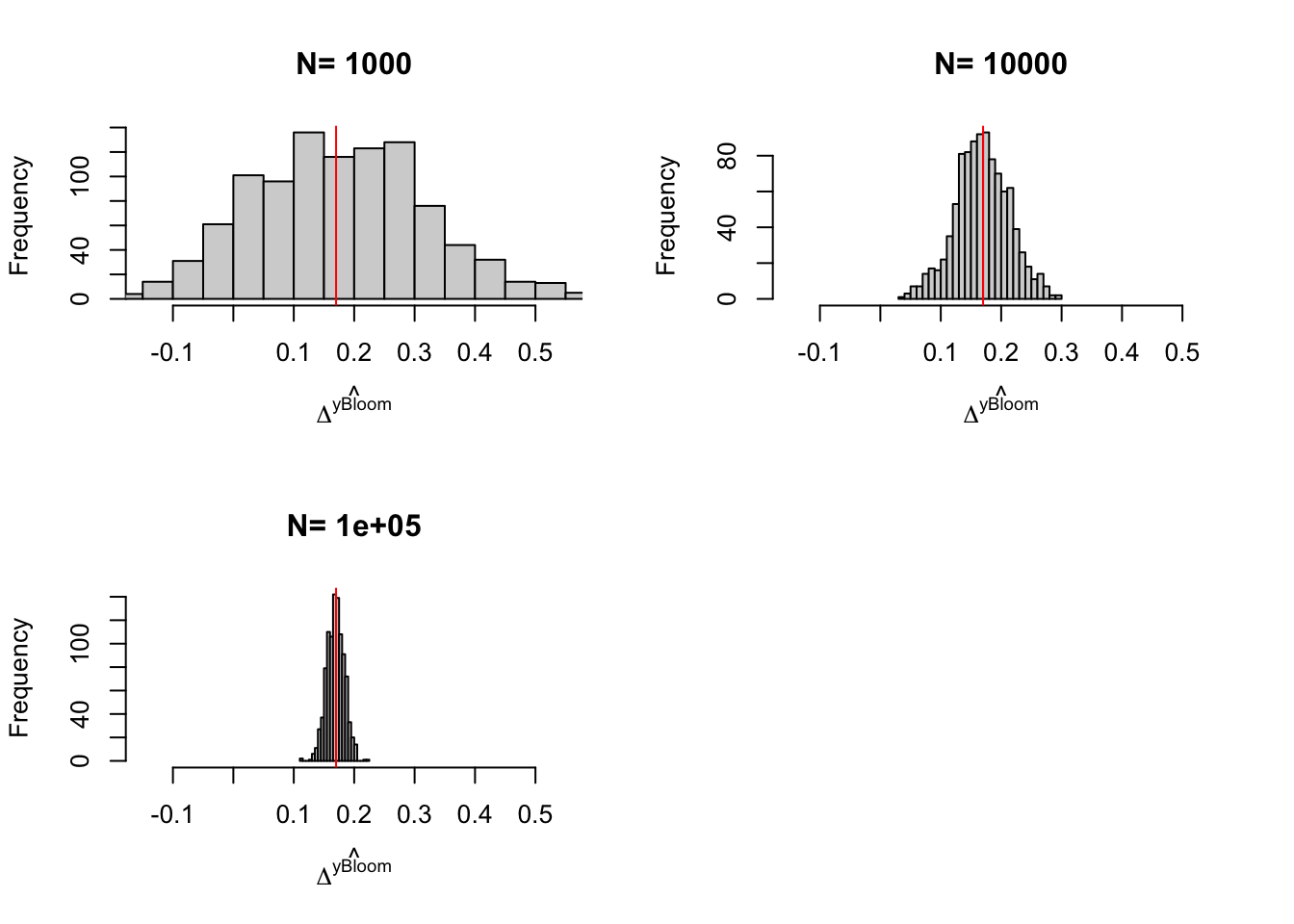
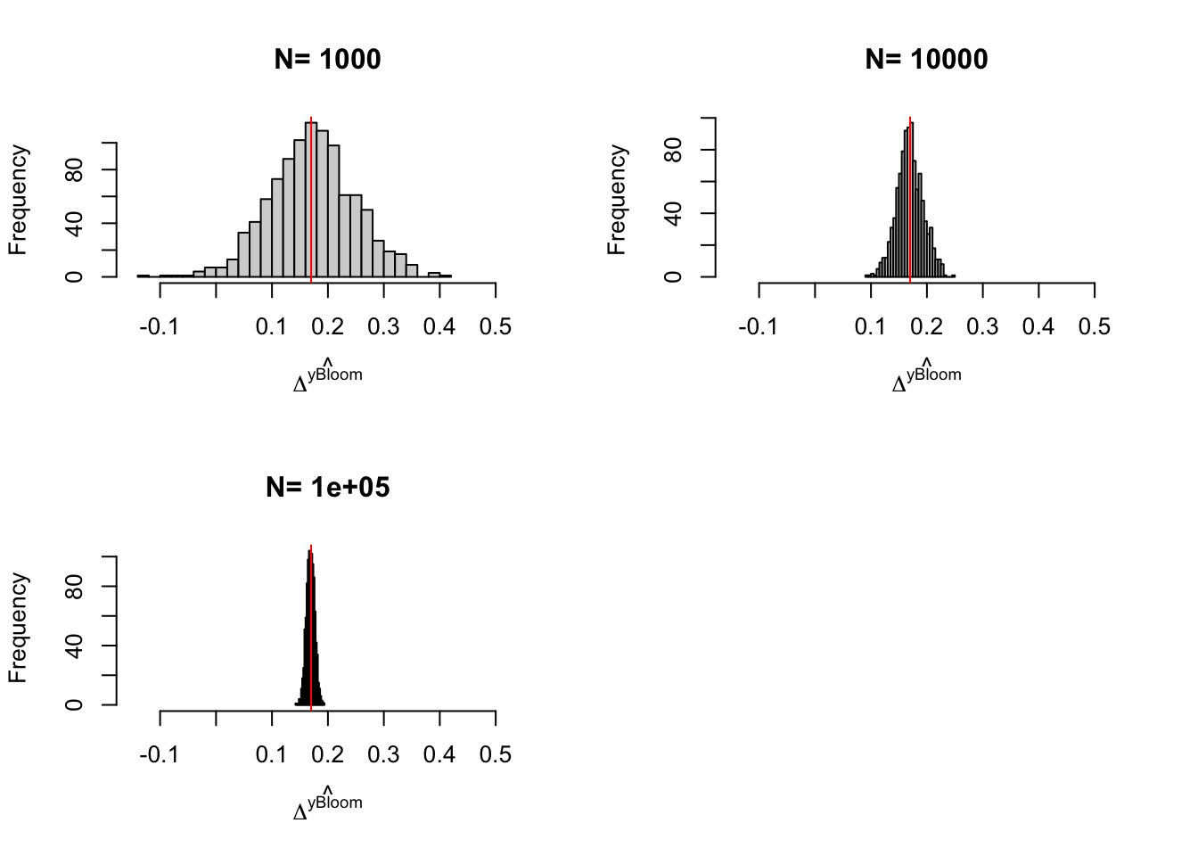
Figure 3.6: Distribution of the \(Bloom\) and \(Bloom(X)\) estimators with randomization after eligibility over replications of samples of different sizes
We can take three things from Figure 3.6:
- Problems with the IV estimator appear with \(N=100\) (probably because there are some samples where no one is treated).
- Sampling noise from randomization after eligibility is indeed larger than sampling noise from Self-Selection design.
- Conditioning on covariates helps.
3.3.3 Estimating sampling noise
As always, we can estimate samling noise either using the CLT or resampling methods. Using the CLT, we can derive the following formula for the distribution of the Bloom estimator:
Theorem 3.8 (Asymptotic Distribution of $\hat{\Delta}^Y_{Bloom}$) Under Assumptions 3.5, 3.6 and 3.7 and assuming that there is at least one individual with \(R_i=1\) and one individual with \(D_i=1\), we have (keeping the conditioning on \(E_i=1\) implicit):
\[\begin{align*} \sqrt{N}(\hat{\Delta}^Y_{Bloom}-\Delta^Y_{TT}) & \stackrel{d}{\rightarrow} \mathcal{N}\left(0,\frac{1}{(p^{D}_1)^2}\left[\left(\frac{p^D}{p^R}\right)^2\frac{\var{Y_i|R_i=0}}{1-p^R}+\left(\frac{1-p^D}{1-p^R}\right)^2\frac{\var{Y_i|R_i=1}}{p^R}\right]\right), \end{align*}\]
with \(p^D=\Pr(D_i=1)\), \(p^R=\Pr(R_i=1)\) and \((p^{D}_1=\Pr(D_i=1|R_i=1)\).
Proof. The proof is immediate using Theorem 3.16, setting \(p^{AT}=0\).
Remark. Theorem 3.8 shows that there is a price to pay for not randomizing after self-selection. This price is a decrease in precision. The variance of the estimator is weighted by \(\frac{1}{(\Pr(D_i=1|R_i=1))^2}\). This means that the effective sample size is equal to the number of individuals that take up the treatment when offered. We generaly call these individuals “compliers,” since they comply with the treatment assignment. Sampling noise is of the same order of magnitude as the number of compliers You might have very low precision despite a very large sample size if you have a very small proportion of compliers.
Remark. In order to compute an estimate of the sampling noise of the Bloom estimator, we can either use the plug-in formula from Theorem 3.8 or use the IV standard errors robust to heteroskedasticity. Here is a simple function in order to compute the plug-in estimator:
var.RAE.plugin <- function(pD1,pD,pR,V0,V1,N){
  return(((pD/pR)^2*(V0/(1-pR))+((1-pD)/(1-pR))^2*(V1/pR))/(N*pD1^2))
}
Example 3.21 Let us derive the CLT-based estimates of sampling noise using both the plug-in estimator and the IV standard errors without conditioning on covariates first. For the sake of the example, I’m working with a sample of size \(N=1000\).
sn.RAE.simuls <- 2*quantile(abs(simuls.elig[['1000']][,'Bloom']-delta.y.tt),probs=c(0.99))
sn.RAE.IV.plugin <- 2*qnorm((.99+1)/2)*sqrt(var.RAE.plugin(pD1=mean(Ds[E==1 & R==1]),pD=mean(Ds[E==1]),pR=mean(R[E==1]),V0=var(y[R==0 & E==1]),V1=var(y[R==1 & E==1]),N=length(y[E==1])))
sn.RAE.IV.homo <- 2*qnorm((.99+1)/2)*sqrt(vcov(reg.y.R.2sls.elig)[2,2])
sn.RAE.IV.hetero <- 2*qnorm((.99+1)/2)*sqrt(vcovHC(reg.y.R.2sls.elig,type='HC2')[2,2])
True 99% sampling noise (from the simulations) is 0.757. 99% sampling noise estimated using the plug-in estimator is 0.921. 99% sampling noise estimated using default IV standard errors is 1.069. 99% sampling noise estimated using heteroskedasticity robust IV standard errors is 0.92.
Conditioning on covariates:
sn.RAE.simuls.yB <- 2*quantile(abs(simuls.elig.yB[['1000']][,'Bloom']-delta.y.tt),probs=c(0.99))
sn.RAE.IV.homo.yB <- 2*qnorm((.99+1)/2)*sqrt(vcov(reg.y.R.yB.2sls.elig)[2,2])
sn.RAE.IV.hetero.yB <- 2*qnorm((.99+1)/2)*sqrt(vcovHC(reg.y.R.yB.2sls.elig,type='HC2')[2,2])
True 99% sampling noise (from the simulations) is 0.393. 99% sampling noise estimated using default IV standard errors is 0.457. 99% sampling noise estimated using heteroskedasticity robust IV standard errors is 0.454.
Remark. Sampling noise in the Randomization After Eligibility design seems larger than sampling noise in the Self-Selection design.
In the Self-Selection design, sampling noise with \(N=1000\) is equal to 0.55. In the Eligibility design, sampling noise with \(N=1000\) is equal to 0.76. Why such a difference? Both designs have the same effective sample size.
In the Self-Selection design, the effective sample size \(N^{SS}_e\) is the number of eligible individuals that apply to take up the program: \(N^{SS}_e=N\Pr(D_i=1|E_i=1)\Pr(E_i=1)\). In our example, \(N^{SS}_e=1000 *\) 0.459 \(*\) 0.218 \(=\) 100.
In the Eligibility design, the sample size on which the regressions are performed is \(N^{E}\), the number of eligible individuals: \(N^{E}=N\Pr(E_i=1)\). In our example, \(N^{E}=1000 *\) 0.459 \(=\) 459. But the effective sample size for the Randomization After Eligibility design is actually equal to the one in the Self-Selection design because only compliers matter for the precision of the Bloom estimator, as Theorem 3.8 shows. Thus \(N^{SS}_e=N^{E}_e\).
Why then is sampling noise much larger in the Randomization After Eligibility design? Probably because the Bloom estimator cannot enforce the fact that the impact of the program on non compliers is zero. It has to estimate the average outcome of non compliers in both treatment arms and hope that they cancel. In real samples, they won’t, increasing the size of sampling noise.
3.4 Encouragement Design
In an Encouragement Design, we randomly select two groups among the eligibles, as in Randomization After Eligibility. Treated individuals randomly receive an encouragement to participate in the program and decide whether they want to comply with the encouragement and join the program. Individuals in the control group do not receive an encouragement, but they can still decide to self-select in the program. The Encouragement design differs from the Randomization After Eligibility design mainly by not barring entry into the programs to individuals in the control group. If successful, the encouragement generates a higher level of take up of the program in the treatment group than in the control group. Examples of encouragements are additional reminders that the program exists, help in subscribing the program, financial incentives for subscribing the program, etc.
In an Encouragement Design, we can recover the causal effect of the treatment not on all the treated but on the treated whose participation into the program has been triggered by the encouragement. The individuals reacting to the encouragement by participating in the program are usually called compliers. The effect of the treatment on the compliers is called the Local Average Treatment Effect. The main identification result for Encouragement designs is that a Wald ratio (an IV estimator) recovers the LATE. It is due to Imbens and Angrist (1994). A key assumption for this result is exclusion restriction: there has to be zero impact of the encouragement on the outcome, except through participation in the treatment. A second key assumption is that no one individual is driven away from participating in the treatment because of the encouragement. This assumption is called monotonicity.
Let’s detail these assumptions, the identification result and the estimation strategy.
3.4.1 Identification
3.4.1.1 Identification of the Local Average Treatment Effect
Before stating the identification results, let’s go through some definitions and assumptions. We are going to denote \(R_i=1\) when individual \(i\) receives the encouragement and \(R_i=0\) when she does not. As in Section 3.3, we have four potential outcomes for \(Y_i\): \(Y_i^{d,r}\), \((d,r)\in\left\{0,1\right\}^2\), where \(d\) denotes receiving the treatment and \(r\) receiving the encouragement. We also have two potential outcomes for \(D_i\): \(D_i^{r}\), \(r\in\left\{0,1\right\}\). \(D_i^{1}\) indicates whether individual \(i\) takes the treatment when receving the encouragement and \(D_i^{0}\) whether she takes the treatment when not receiving the encouragement. These potential outcomes define four possible types of individuals, that I’m going to denote with the random variable \(T_i\):
- Always takers, who take up the program whether they receive the encouragement or not. They are such that \(D_i^{1}=D_i^{0}=1\). I denote them \(T_i=a\).
- Never takers, who do not take up the program whether they receive the encouragement or not. They are such that \(D_i^{1}=D_i^{0}=0\). I denote them \(T_i=n\).
- Compliers, who take up the program when they receive the encouragement and do not when they do not receive the encouragement. They are such that \(D_i^{1}-D_i^{0}=1\). I denote them \(T_i=c\).
- Defiers, who do not take up the program when they receive the encouragement and take it up when they do not receive the encouragement. They are such that \(D_i^{1}-D_i^{0}=-1\). I denote them \(T_i=d\).
We are now ready to state the assumptions needed for identification of the LATE.
Definition 3.9 (Encouragement Validity) We assume that the randomized allocation of the program does not interfere with how potential outcomes and self-selection are generated:
\[\begin{align*} D_i & = D_i^1R_i+(1-R_i)D_i^0 \\ Y_i & = \begin{cases} Y_i^{1,1} & \text{ if } (R_i=1 \text{ and } D_i=1) \\ Y_i^{0,1} & \text{ if } (R_i=1 \text{ and } D_i=0) \\ Y_i^{1,0} & \text{ if } (R_i=0 \text{ and } D_i=1) \\ Y_i^{0,0} & \text{ if } (R_i=0 \text{ and } D_i=0) \end{cases} \end{align*}\]
with \(Y_i^{1,1}\), \(Y_i^{0,1}\), \(Y_i^{1,0}\), \(Y_i^{0,0}\), \(D_i^1\) and \(D^0_i\) the same potential outcomes and self-selection decisions as in a routine allocation of the treatment.
Definition 3.10 (Independence of Encouragement) We assume that the randomized allocation of the program is well done:
\[\begin{align*} (Y_i^{1,1},Y_i^{0,1},Y_i^{0,0},Y_i^{1,0},D_i^1,D^0_i)\Ind R_i|E_i=1. \end{align*}\]
Definition 3.11 (Exclusion Restriction) We assume that the randomized allocation of the program does not alter potential outcomes:
\[\begin{align*} Y_i^{d,r} & = Y_i^d \text{, }\forall (r,d)\in\left\{0,1\right\}^2. \end{align*}\]
Definition 3.12 (First Stage) We assume that the encouragement does manage to increase participation:
\[\begin{align*} \Pr(D_i=1|R_i=1,E_i=1) > \Pr(D_i=1|R_i=0,E_i=1). \end{align*}\]
Definition 3.13 (Monotonicity) We assume that the encouragement either increases participation for everyone or decreases participation for everyone:
\[\begin{align*} \text{ either } \forall i\text{, }D_i^1\geq D_i^0 \text{ or } \forall i\text{, }D_i^1\leq D_i^0 . \end{align*}\]
Assumption 3.13 means that we cannot have simultaneously individuals that are pushed by the encouragement into the treatment and individuals that are pushed out of the treatment. As a consequence, there cannot be compliers and defiers at the same time. There can only be compliers or defiers. For simplicity, in what follows, I assume that there are no defiers. This is without loss of generality, since, under Assumption 3.13, a redefinition of the treatment (\(\tilde{D}_i=-D_i\)) moves the model in this section from one with only defiers to one with only compliers.
Theorem 3.9 (Identification in an Encouragement Design) Under Assumptions 3.9, 3.10, 3.11, 3.12 and 3.13, the Wald estimator identifies the LATE:
\[\begin{align*} \Delta^Y_{Wald} & = \Delta^Y_{LATE}, \end{align*}\]
with:
\[\begin{align*} \Delta^Y_{Wald} & = \frac{\esp{Y_i|R_i=1,E_i=1} - \esp{Y_i|R_i=0,E_i=1}}{\Pr(D_i=1|R_i=1,E_i=1)-\Pr(D_i=1|R_i=0,E_i=1)}\\ \Delta^Y_{LATE} & = \esp{Y^1_i-Y^0_i|T_i=c,E_i=1}. \end{align*}\]
Proof. See Section A.2.1.
Remark. Theorem 3.9 is pretty amazing. It shows that there exists a set of assumptions under which we can use an encouragement design to recover the effect of the treatment (\(D_i\)) on outcomes, despite the fact that we have NOT randomized \(D_i\). The assumptions needed for that to happen are intuitive:
- The encouragement has to have no direct effect on the outcomes (Assumption 3.11)
- The encouragement has to have an effect on treatment uptake (Assumption 3.12)
- The encouragement does not generate two-way flows in and out of the treatment, but only a one-way flow (Assumption 3.13)
Under these assumptions, the only way that we can see a difference in outcomes between those that receive the encouragement and those that do not is that the treatment has had an effect on those that have taken it because of the encouragement. It cannot be because of the encouragement itself, because of Assumption 3.11. It cannot be because some people with particularly low outcomes have exited the program because of the encouragement, Assumption 3.13 forbids it. And if we see no effect of the encouragement, it has to be that the treatment has no effect on the compliers as well, because Assumption 3.12 implies that they have received the treatment in the encouragement group and that they have not in the group without encouragement.
Remark. Less nice with Theorem 3.9 is that we recover the effect only for a subgroup of individuals, the compliers. This raises two issues:
- The effect on the compliers (or LATE) is not the effect on the treated (TT). When the treatment is given in routine mode, without the encouragement, TT is actually equal to the effect on the always takers. There is nothing that tells us that the always takers react in the same way to the treatment as the compliers. As soon as the expected benefits of the treatment enter the decision of taking it up, always takers have larger treatment effects than compliers.
- The identity of the compliers is unobserved. We cannot decide to allocate the treatment only to the compliers because they are defined by their counterfactual response to the encouragement. In both treatment arms, we do not know who the compliers are. We know they are among those who take up the program in the group receiving the encouragement. But there are also always takers that take up the program in this group. We know that they are among those that do not take up the program in the group that does not receive the encouragement. But never takers behave in the same way in that group.
The only way to direct the treatment at the compliers is to use the encouragement. So, we end up evaluating the effect of the encouragement itself and not of the program. In that case, we do not need Assumptions 3.11, 3.12 and 3.13, because they are not needed to identify the effect of the encouragement (see Section 3.4.1.2 below).
In general, researchers believe that LATE tells them something about the magnitude of the effect beyond compliers. This is not warranted by the maths, but one can understand how a bayesian decision-maker may use the information from some subpopulation to infer what would happen to another. Comparing LATEs and TTs for similar treatments is an active area for reasearch. I know of no paper doing that extensively and nicely.
To generalize from the LATE to the TT, we can make the assumption that the impact on always takers is equal to the impact on compliers, but that seems a little far-fetched. Angrist and Fernandez-Val propose to assume that the effect on compliers is equal to the effect on always takers conditional on some observed covariates. When outcomes are bounded (for example because they are between zero and one), we can try to bound the \(TT\) using the \(LATE\) (see Huber, Laffers and Mellace (2017)).
Remark. If you see a connexion between the conditions for the Wald estimator to identify LATE and the assumptions behind an IV estimator, you’re correct. The Wald estimator is actually an IV estimator (see Theorem 3.15 below).
3.4.1.2 Identification of the Intention to Treat Effect
In this section, we are going to delineate how to identify the Intention to Treat Effect (ITE) in an Encouragement design. In an Encouragement design, ITE is the effect of receiving the encouragement. It is defined in a similar manner as in a Randomization After Eligibility design (see Definition 3.8): \(\Delta^Y_{ITE} = \esp{Y_i^{D_i^1,1}-Y_i^{D_i^0,0}|E_i=1}\).
Under Assumption 3.9, receiving the encouragement has several impacts:
- Some individuals (the compliers) decide to enter the program,
- Some individuals (the defiers) decide to exit the program,
- The encouragement might have a direct effect on outcomes (\(Y_i^{d,1}\neq Y_i^{d,0}\)).
This last effect is the effect of receiving the encouragement that does not goes through participation into the program. For example, it is possible that sending an encouragement to take up a retirement program makes me save more for retirement, even if I end up not taking up the proposed program.
The two causal channels that are at work within the ITE can be seen more clearly when decomposing the ITE to make each type appear. We can do that because the four types define a partition of the sample space, that is a collection of mutually exclusive events whose union spans the whole space. As a consequence of that, conditioning on the union of the four types is the same thing as not conditioning on anything. Using this trick, we have:
\[\begin{align} \Delta^Y_{ITE} & = \esp{Y_i^{D_i^1,1}-Y_i^{D_i^0,0}|(T_i=a\cup T_i=c\cup T_i=d\cup T_i=n)\cap E_i=1}\nonumber\\ & = \esp{Y_i^{D_i^1,1}-Y_i^{D_i^0,0}|T_i=a,E_i=1}\Pr(T_i=a|E_i=1)\nonumber\\ & \phantom{=}+ \esp{Y_i^{D_i^1,1}-Y_i^{D_i^0,0}|T_i=c,E_i=1}\Pr(T_i=c|E_i=1)\nonumber\\ & \phantom{=}+ \esp{Y_i^{D_i^1,1}-Y_i^{D_i^0,0}|T_i=d,E_i=1}\Pr(T_i=d|E_i=1)\nonumber\\ & \phantom{=}+ \esp{Y_i^{D_i^1,1}-Y_i^{D_i^0,0}|T_i=n,E_i=1}\Pr(T_i=n|E_i=1)\nonumber\\ & = \esp{Y_i^{1,1}-Y_i^{1,0}|T_i=a,E_i=1}\Pr(T_i=a|E_i=1)\nonumber\\ & \phantom{=}+ \esp{Y_i^{1,1}-Y_i^{0,0}|T_i=c,E_i=1}\Pr(T_i=c|E_i=1)\nonumber\\ & \phantom{=}+ \esp{Y_i^{0,1}-Y_i^{1,0}|T_i=d,E_i=1}\Pr(T_i=d|E_i=1)\nonumber\\ & \phantom{=}+ \esp{Y_i^{0,1}-Y_i^{0,0}|T_i=n,E_i=1}\Pr(T_i=n|E_i=1),\tag{3.2} \end{align}\]
where the first equality follows from the four types defining a partition of the sample space, the second equality from the usual rule of conditional expectations and the fact that types are disjoint events, and the third equality from Assumption 3.6.
We can now see that ITE is composed of four terms:
- The effect of receiving the encouragment on the always takers. This effect is only the direct effect of the encouragement, and not the effect of the program since the always takers always take the program. This term cancels under Assumption 3.11, when there is no direct effect of the encouragement on outcomes.
- The effect of receiving the encouragement on compliers. This is both the effect of the encouragement and of the program. This is equal to the LATE under Assumption 3.11.
- The effect of receiving the encouragement on defiers. This is the difference between the direct effect of the encouragement and the effect of the program. This is equal to the opposite of the effect of the treatment on the defiers under Assumption 3.11.
- The effect of receiving the encouragement on never takers. This effect is only the direct effect of the encouragement, and not the effect of the program since the never takers never take the program. This term cancels under Assumption 3.11.
All these effects are weighted by the respective proportions of the types in the population. ITE is linked to LATE. This link can be made clearer:
Theorem 3.10 (From ITE to Compliers and Defiers) Under Assumptions 3.9 and 3.11, ITE is equal to the effect on compliers minus the effect on defiers weighted by their respective proportions in the population:
\[\begin{align*} \Delta^Y_{ITE} & = \esp{Y_i^{1}-Y_i^{0}|T_i=c,E_i=1}\Pr(T_i=c|E_i=1)\\ & \phantom{=}-\esp{Y_i^{1}-Y_i^{0}|T_i=d,E_i=1}\Pr(T_i=d|E_i=1). \end{align*}\]
Proof. Under Assumption 3.11, Equation (3.2) becomes:
\[\begin{align*} \Delta^Y_{ITE} & = \esp{Y_i^{1}-Y_i^{1}|T_i=a,E_i=1}\Pr(T_i=a|E_i=1)\\ & \phantom{=}+ \esp{Y_i^{1}-Y_i^{0}|T_i=c,E_i=1}\Pr(T_i=c|E_i=1)\\ & \phantom{=}+ \esp{Y_i^{0}-Y_i^{1}|T_i=d,E_i=1}\Pr(T_i=d|E_i=1)\\ & \phantom{=}+ \esp{Y_i^{0}-Y_i^{0}|T_i=n,E_i=1}\Pr(T_i=n|E_i=1) \end{align*}\]
which proves the result.
The previous theorem shows that Assumption 3.11 shuts down any direct effect of receiving the encouragement on outcomes. As a consequence of this assumption, the only impact that receiving the encouragement has on outcomes is through participation into the program. Hence, ITE is equal to the impact of the program on those who react to the encouragement: the compliers and the defiers, weighted by their respective proportions.
The problem with the result of Theorem 3.10 is that ITE contains two-way flows in and out of the program. If we want to know something about the effect of the program, and not only about the effect of the encouragement, we need to assume that defiers do not exist. That’s what Assumption 3.13 does, as the following theorem shows:
Theorem 3.11 (From ITE to LATE) Under Assumptions 3.9, 3.11 and 3.13, ITE is equal to the LATE multiplied by the proportion of compliers in the population:
\[\begin{align*} \Delta^Y_{ITE} & = \Delta^Y_{LATE}\Pr(T_i=c|E_i=1). \end{align*}\]
Proof. The result is straighforward using Assumption 3.13 and Theorem 3.10. Indeed, Assumption 3.13 implies that \(\forall i\), \(D_i^1-D_i^0\geq 0\) (choosing only the first “either” statement, without loss of generality). As a consequence, \(\Pr(T_i=d|E_i=1)=\Pr(D_i^1-D_i^0=-1|E_i=1)=0\).
In order to move from the link between LATE and ITE to the mechanics of the Wald estimator, we need two additional identification results. The first result shows that ITE can be identified under fairly light conditions by a WW estimator. The second result shows that the proportion of people taking up the treatment when eligiblity is announced is also easily estimated from the data.
Theorem 3.12 (Identification of ITE in an Encouragement Design) Under Assumptions 3.9 and 3.10, ITE is identified by the With/Without comparison among eligibles:
\[\begin{align*} \Delta^Y_{ITE} & = \Delta^Y_{WW|E_i=1}. \end{align*}\]
Proof. \[\begin{align*} \Delta^Y_{WW|E=1} & =\esp{Y_i|R_i=1,E_i=1}-\esp{Y_i|R_i=0,E_i=1} \\ & = \esp{Y_i^{D_i^1,1}|R_i=1,E_i=1}-\esp{Y_i^{D_i^0,0}|R_i=0,E_i=1} \\ & = \esp{Y_i^{D_i^1,1}|E_i=1}-\esp{Y_i^{D_i^0,0}|E_i=1}, \end{align*}\] where the second equality follows from Assumption 3.9 and the third from Assumption 3.10.
Theorem 3.13 (Identification of the Proportion of Compliers) Under Assumptions 3.9, 3.10 and 3.13, the proportion of compliers is identified by the difference between the proportion of people taking up the program among those receiving the encouragement and the proportion of individuals taking up the program among those not receiving the encouragement:
\[\begin{align*} \Pr(T_i=c|E_i=1) & = \Pr(D_i=1|R_i=1,E_i=1)-\Pr(D_i=1|R_i=0,E_i=1). \end{align*}\]
Proof. \[\begin{align*} \Pr(D_i=1|R_i=1,E_i=1) & =\Pr(D_i=1\cap (T_i=a\cup T_i=c\cup T_i=d\cup T_i=n)|R_i=1,E_i=1) \\ & = \Pr(D_i=1\cap T_i=a|R_i=1,E_i=1)\\ & \phantom{=}+ \Pr(D_i=1\cap T_i=c|R_i=1,E_i=1)\\ & \phantom{=} +\Pr(D_i=1\cap T_i=d|R_i=1,E_i=1)\\ & \phantom{=} +\Pr(D_i=1\cap T_i=n|R_i=1,E_i=1)\\ & = \Pr(T_i=a|R_i=1,E_i=1)\\ & \phantom{=} +\Pr(T_i=c|R_i=1,E_i=1)\\ & = \Pr(T_i=a|E_i=1)\\ & \phantom{=} +\Pr(T_i=c|E_i=1), \end{align*}\]
where the first equality follows the types being a partition of the sample space; the second equality from the fact that the types are disjoint sets; the third equality from the fact that \(T_i=a|R_i=1 \Rightarrow D_i=1\) (so that \(\Pr(D_i=1\cap T_i=a|R_i=1,E_i=1)=\Pr(T_i=a|R_i=1,E_i=1)\)), \(T_i=c|R_i=1 \Rightarrow D_i=1\) (so that \(\Pr(D_i=1\cap T_i=c|R_i=1,E_i=1)=\Pr(T_i=c|R_i=1,E_i=1)\)), \(T_i=d|R_i=1 \Rightarrow D_i=0\) (so that \(\Pr(D_i=1\cap T_i=d|R_i=1,E_i=1)=0\)) and \(T_i=n|R_i=1 \Rightarrow D_i=0\) (so that \(\Pr(D_i=1\cap T_i=n|R_i=1,E_i=1)=0\)); and the fourth equality from Assumption 3.10 and Lemma A.6.
Corollary 3.2 (Wald estimator and ITE) It follows from Theorems 3.12 and 3.13 that, under Assumptions 3.9, 3.10 and 3.13, the Wald estimator is equal to the ITE divided by the propotion of compliers:
\[\begin{align*} \Delta^Y_{Wald|E=1} & = \frac{\Delta^Y_{ITE}}{\Pr(T_i=c|E_i=1)}. \end{align*}\]
As a consequence of Corollary 3.2, we see that the Wald estimator reweights the ITE, the effect of receiving an encouragement, by the proportion of people reacting to the encouragement by participating in the program, the compliers. From Theorem 3.10, we know that this ratio will be equal to LATE if the Assumption 3.11 also holds, so that all the impact of the encouragement stems from entering the program. The encouragement serves as an instrument for program participation.
Remark. The Encouragement design seems like magic. You do not assign randomly the program, but only an encouragement to take it, and you can recover the effect of the program anyway. The Encouragement design is less intrusive than the Self-Selection and Eligibility designs. In an Encouragement design, you do not have to refuse the program to agents in the control group. You pay two types of prices for that:
- You only recover LATE, not TT
- You have larger sampling noise.
The intuition for this second point can be delineated using the very same apparatus that we have developed so far. So here goes. Under the assumptions made so far, it is easy to show that (omitting the conditioning on \(E_i=1\) for simplicity):
\[\begin{align*} \Delta^Y_{WW|E=1} & = \esp{Y_i^{1,1}|T_i=a,R_i=1}\Pr(T_i=a,|R_i=1)\\ & \phantom{=}-\esp{Y_i^{1,0}|T_i=a,R_i=0}\Pr(T_i=a,|R_i=0)\\ & \phantom{=}+ \esp{Y_i^{1,1}|T_i=c,R_i=1}\Pr(T_i=c|R_i=1)\\ & \phantom{=}-\esp{Y_i^{0,0}|T_i=c,R_i=0}\Pr(T_i=c|R_i=0)\\ & \phantom{=}+ \esp{Y_i^{0,1}|T_i=d,R_i=1}\Pr(T_i=d|R_i=1)\\ & \phantom{=}-\esp{Y_i^{1,0}|T_i=d,R_i=0}\Pr(T_i=d|R_i=0)\\ & \phantom{=}+ \esp{Y_i^{0,1}|T_i=n,R_i=1}\Pr(T_i=n|R_i=1)\\ & \phantom{=}-\esp{Y_i^{0,0}|T_i=n,R_i=0}\Pr(T_i=n|R_i=0). \end{align*}\]
The four parts of the equation account for comparisons among each type between the two treatment arms. The parts due to always takers and never takers cancel out under Assumptions 3.10 and 3.11. But this cancelling out only happens in the population. In a given sample, the sample equivalents of the two members of each difference do not have to be equal, and thus they do not cancel out, generating sampling noise. Ideally, we would like to enforce that the effect of the encouragement on always takers and never takers is null, as Assumption 3.11 imposes, but that would require observing the type variable \(T_i\). Unfortunately, we cannot now the type of each individual in the sample, since it is defined counterfactually. Maybe someday we’ll be able to use prior responses to the encouragement to identify the type of each individual and thus improve the precision of the Wald estimator.
Explain de Chaisemartin.
Remark. what if we fear there are defiers. de Chaisemartin
Remark. In practice, we use a pseudo-RNG to allocate the randomized annoucement of the encouragement:
\[\begin{align*} R_i^* & \sim \mathcal{U}[0,1]\\ R_i & = \begin{cases} 1 & \text{ if } R_i^*\leq .5 \land E_i=1\\ 0 & \text{ if } R_i^*> .5 \land E_i=1 \end{cases} \\ D_i & = \uns{\bar{\alpha}+\theta\bar{\mu}+\psi R_i-C_i\geq0 \land E_i=1} \end{align*}\]
\(\psi\) denotes the increase in agents’ valuation of the program after receiving the encouragement.
Example 3.22 Let’s see how the encouragement design works in our numerical example. Let’s choose a value for \(\psi\) and add it to the vector of parameters.
param <- c(param,0.6)
names(param) <- c("barmu","sigma2mu","sigma2U","barY","rho","theta","sigma2epsilon","sigma2eta","delta","baralpha","barc","gamma","sigma2V","psi")
Let’s first compute the value of LATE in this new model. Let’s denote \(D_i^{*0}=\bar{\alpha}+\theta\bar{\mu}-C_i\) the utility of agent \(i\) absent the encouragement, with \(C_i=\bar{c} + \gamma \mu_i + V_i\). In order to be a complier, you have to have a utility of the program that is insufficient to make you apply for the program when you receive no encouragement (\(D_i^{*0}<0\)) and a positive utility of applying to the treatment after receiving the encouragement (\(D_i^{*0}+\psi\geq 0\)). Compliers are thus such that \(-\psi\leq D_i^{*0}<0\). LATE can thus be written as follows in our model:
\[\begin{align*} \Delta^y_{LATE} & = \bar{\alpha}+ \theta\esp{\mu_i|\mu_i+U_i^B\leq\bar{y} \land -\psi\leq D_i^{*0}<0}, \end{align*}\]
Using the same approach, we can also compute the proportion of compliers among eligibles. In our model, we indeed have:
\[\begin{align*} \Pr(T_i=c|E_i=1) & = \Pr(-\psi\leq D_i^{*0}<0|\mu_i+U_i^B\leq\bar{y}). \end{align*}\]
Since all errors terms are normally distributed in our model, we can compute the package tmvtnorm to compute both LATE and the proportion of compliers among eligibles.
\[\begin{align*} (\mu_i,y_i^B,D_i^{*0}) & \sim \mathcal{N}\left(\bar{\mu},\bar{\mu},\bar{\alpha}+(\theta-\gamma)\bar{\mu}-\bar{c}, \left(\begin{array}{ccc} \sigma^2_{\mu} & \sigma^2_{\mu} & -\gamma\sigma^2_{\mu} \\ \sigma^2_{\mu} & \sigma^2_{\mu} + \sigma^2_{U} & -\gamma\sigma^2_{\mu} \\ -\gamma\sigma^2_{\mu} & -\gamma\sigma^2_{\mu} & \gamma^2\sigma^2_{\mu}+\sigma^2_{V} \end{array} \right) \right) \end{align*}\]
mean.mu.yB.Dstar <- c(param['barmu'],param['barmu'],param['baralpha']- param['barc']+(param['theta']-param['gamma'])*param['barmu'])
cov.mu.yB.Dstar <- matrix(c(param['sigma2mu'],param["sigma2mu"],-param['gamma']*param["sigma2mu"],
                            param["sigma2mu"],param['sigma2mu']+param['sigma2U'],-param['gamma']*param["sigma2mu"],
                            -param['gamma']*param["sigma2mu"],-param['gamma']*param["sigma2mu"],param["sigma2mu"]*(param['gamma'])^2+param['sigma2V']),3,3,byrow=TRUE)
# late
lower.cut <- c(-Inf,-Inf,-param['psi'])
upper.cut <- c(Inf,log(param['barY']),0)
moments.cut <- mtmvnorm(mean=mean.mu.yB.Dstar,sigma=cov.mu.yB.Dstar,lower=lower.cut,upper=upper.cut)
delta.y.late <- param['baralpha']+ param['theta']*moments.cut$tmean[1]
# proportion of compliers
lower.cut <- c(-Inf,-Inf,-Inf)
upper.cut <- c(Inf,log(param['barY']),Inf)
pr.compliers <- ptmvnorm.marginal(xn=0,n=3,mean=mean.mu.yB.Dstar,sigma=cov.mu.yB.Dstar,lower=lower.cut,upper=upper.cut)-ptmvnorm.marginal(xn=-param['psi'],n=3,mean=mean.mu.yB.Dstar,sigma=cov.mu.yB.Dstar,lower=lower.cut,upper=upper.cut)
delta.y.ite <- delta.y.late*pr.compliers
The value of \(\Delta^y_{LATE}\) in the population is thus 0.173. The proportion of compliers among eligibles in the population is 0.272. As a consequence of Corollary 3.2, we can compute ITE as the product of LATE and the proportion of compliers. In our example, ITE is thus equal to 0.047 in the population.
Now let’s simulate a new sample with the encouragement delivered randomly among eligibles. I’m also defining the potential outcomes \(D^1_i\) and \(D^0_i\) and the types \(T_i\) for later use.
# I'm changing the seed because with the usual one, I get a negative estimate of the treatment effect: lots of sampling noise!
set.seed(12345)
N <-1000
mu <- rnorm(N,param["barmu"],sqrt(param["sigma2mu"]))
UB <- rnorm(N,0,sqrt(param["sigma2U"]))
yB <- mu + UB
YB <- exp(yB)
epsilon <- rnorm(N,0,sqrt(param["sigma2epsilon"]))
eta<- rnorm(N,0,sqrt(param["sigma2eta"]))
U0 <- param["rho"]*UB + epsilon
y0 <- mu +  U0 + param["delta"]
alpha <- param["baralpha"]+  param["theta"]*mu + eta
y1 <- y0+alpha
Y0 <- exp(y0)
Y1 <- exp(y1)

#random allocation of encouragement among eligibles
E <- ifelse(YB<=param["barY"],1,0)
Rs <- runif(N)
R <- ifelse(Rs<=.5 & E==1,1,0)
V <- rnorm(N,0,param["sigma2V"])
Dindex <- param["baralpha"]+param["theta"]*param["barmu"]+param["psi"]*R-param["barc"]-param["gamma"]*mu-V
Ds <- ifelse(Dindex>=0 & E==1,1,0)
y <- y1*Ds+y0*(1-Ds)
Y <- Y1*Ds+Y0*(1-Ds)
D <- Ds

# types
Dindex1 <- param["baralpha"]+param["theta"]*param["barmu"]+param["psi"]-param["barc"]-param["gamma"]*mu-V
Dindex0 <- param["baralpha"]+param["theta"]*param["barmu"]-param["barc"]-param["gamma"]*mu-V
D1 <- ifelse(Dindex1>=0 & E==1,1,0)
D0 <- ifelse(Dindex0>=0 & E==1,1,0)
AT <- ifelse(D1==1 & D0==1,1,0)
NT <- ifelse(D1==0 & D0==0,1,0)
Co <- ifelse(D1==1 & D0==0,1,0)

# figures
Ncompliers <- sum(Co)
NElig <- sum(E)
PrCoElig <- Ncompliers/NElig
LATEs <- mean(alpha[Co==1])
ITEs <- LATEs*PrCoElig
In our sample of \(N=\) 1000 individuals, there are only 216 eligibles, and among them 67 compliers. The proportion of compliers among eligibles is thus 0.31. Sample size decreases fast in an encouragement design. The sample LATE is equal to 0.14. The sample ITE is equal to 0.044.
3.4.2 Estimating the Local Average Treatment Effect and the Intention to Treat Effect
Classically, we present the results of an Encouragement design in three stages:
- We show the first stage regression of \(D_i\) on \(R_i\): this estimates the impact of the encouragement on participation into the program and estimates the proportion of compliers.
- We show the reduced form regression of \(Y_i\) on \(R_i\): this estimates the impact of the encouragement on outcomes, also called ITE.
- We finally show the structural regression of \(Y_i\) on \(D_i\) using \(R_i\) as an instrument, which estimates the LATE.
3.4.2.1 First stage regression
The first stage regression is simply to get an estimate of the effect of the encouragement on participation into the program. If there is no effect of the encouragement on participation, we might as well stop there, since there will be no compliers and no effect to estimate. Note that if we observe an effect on the encouragement on outcomes without any effect on participation, we have to accept the fact that the encouragement might have had a direct effect on outcomes and thus that the exclusion restriction assumption does not hold.
Let’s denote this effect of \(R_i\) on \(D_i\) \(\Delta^{D,R}_{TT}=\esp{D_i^1-D_i^0|R_i=1,E_i=1}\). It is a treatment on the treated since we want to estimate the effect of the cnouragement onthose who have received it. Actually, \(\Delta^{D,R}_{TT}\) is also equal to \(\Delta^{D,R}_{ATE}\), since those who have received the encouragement are a random sample of the eligibles.
How to estimate the effect of \(R_i\) on \(D_i\)? When estimating the effect of the encouragement, we are in a Brute Force design among eligibles, so that the appropriate estimator is the With/Without estimator among eligibles:
Theorem 3.14 (Identification of the First Stage Effect in an Encouragment Design) Under Assumptions 3.9 and 3.10, the WW estimator identifies the First Stage Effect (the effect of \(R_i\) on \(D_i\)): \[\begin{align*} \Delta^{D,R}_{WW} & = \Delta^{D,R}_{TT}. \end{align*}\]
Proof. This is a direct consequence of Theorem 3.1.
As we have seen in Chapter 1, the WW estimator is identical to an OLS estimator: The OLS coefficient \(\beta\) in the following regression: \[\begin{align*} D_i & = \alpha + \beta R_i + U_i \end{align*}\] is thus the \(WW\) estimator.
Finally, the advantage of using OLS other the direct WW comparison is that it gives you a direct estimate of sampling noise (see next section) but also that it enables you to condition on additional covariates in the regression: The OLS coefficient \(\beta\) in the following regression: \[\begin{align*} D_i & = \alpha + \beta R_i + \gamma' X_i + U_i \end{align*}\] is a consistent (and even unbiased) estimate of the ATE.
Center covariates at mean?
Example 3.23 In our numerical example, we can compare all these estimators.
WW.D.R <- mean(D[E==1 & R==1])-mean(D[E==1 & R==0])
reg.D.R.ols <- lm(D[E==1]~R[E==1])
reg.D.R.ols.yB <- lm(D[E==1]~R[E==1]+yB[E==1])
\(\hat{\Delta}^{D,R}_{WW} =\) 0.213, while \(\hat{\Delta}^{D,R}_{OLS}=\) 0.213 which is exactly equal, as expected, to the WW estimator. When controlling for \(y^B_i\), we have: \(\hat{\Delta}^{D,R}_{OLS(y^B)}=\) 0.233.
Under monotonicity, \(\Delta^{D,R}_{TT}\) is equal to the proportion of compliers among eligibles. Indeed, this is the proportion of eligibles that participate when receiving the encouragement and that does not participate when not receiving it. In our example, the proportion of compliers among eligibles is 0.272 in the population and 0.31 in the sample. We are thus underestimating the true proportino of compliers, which is going to make us overestimate the LATE.
3.4.2.2 Reduced form regression
The reduced form regression aims at estimating the ITE, that is the impact of receiving the encouragement on outcomes. From Theorem 3.12, we know that the WW estimator among eligibles identifies the ITE in the population. As a consequence of now classical results, the OLS estimator without control variables is equivalent to the WW estimator and the OLS estimator conditioning on covariates might increase precision.
Example 3.24 In our numerical example, we can compare all these estimators.
WW.y.R <- mean(y[E==1 & R==1])-mean(y[E==1 & R==0])
reg.y.R.ols <- lm(y[E==1]~R[E==1])
reg.y.R.ols.yB <- lm(y[E==1]~R[E==1]+yB[E==1])
\(\hat{\Delta}^{y,R}_{WW} =\) 0.179, while \(\hat{\Delta}^{y,R}_{OLS}=\) 0.179 which is exactly equal, as expected, to the WW estimator. When controlling for \(y^B_i\), we have: \(\hat{\Delta}^{y,R}_{OLS(y^B)}=\) 0.108. In our example, the ITE is 0.047 in the population and 0.044 in the sample. Without conditioning on \(Y_i^B\), we are thus overestimating the true ITE by a lot. The consequence is that we are going to overestimate the LATE as well.
3.4.2.3 Structural regression
There are four ways to compute the LATE:
- We can directly compute the sample equivalent to the Wald estimator defined in Theorem 3.9.
- We can divide our estimate of the ITE by the proportion of compliers, as Corollary 3.2 suggests.
- We can run a regression of \(Y\) on \(D\) using \(R\) as an instrumental variable.
- We can run a regression of \(Y\) on \(D\) using \(R\) as an instrumental variable and controlling for some variables \(X\).
It turns out that, in the absence of control variables, the first three estimators are fully equivalent. Corollary 3.2 has already shown that the first two approaches are equivalent in the population. Theorem 3.15 below shows that the Wald estimator is equivalent to an IV estimator.
For simplicity, in all that follows, I am working only in the subgroup of eligible individuals. That means that I’m setting \(E_i=1\) for everyone, so that \(N\) is the number of eligible individuals.
3.4.2.3.1 Using the Wald estimator
The empirical counterpart to the Wald estimator is the difference in mean outcomes between treatment and controls divided by the difference in participation rates between the two groups:
\[\begin{align*} \hat{\Delta}^Y_{Wald} & = \frac{\frac{1}{\sum_{i=1}^N R_i}\sum_{i=1}^N Y_iR_i-\frac{1}{\sum_{i=1}^N (1-R_i)}\sum_{i=1}^N Y_i(1-R_i)}{\frac{1}{\sum_{i=1}^N R_i}\sum_{i=1}^N D_iR_i-\frac{1}{\sum_{i=1}^N (1-R_i)}\sum_{i=1}^N D_i(1-R_i)} \end{align*}\]
Example 3.25 Let’s check how this works in our numerical example.
mean.y.R.1 <- mean(y[E==1 & R==1])
mean.y.R.0 <- mean(y[E==1 & R==0])
mean.D.R.1 <- mean(D[E==1 & R==1])
mean.D.R.0 <- mean(D[E==1 & R==0])
delta.y.Wald <- (mean.y.R.1-mean.y.R.0)/(mean.D.R.1-mean.D.R.0)
The numerator of the Wald estimator is equal to 7.059 \(-\) 6.88 \(=\) 0.179. The denominator of the Wald estimator is equal to 0.704 \(-\) 0.491 \(=\) 0.213. Overall, the Wald estimator of the LATE is equal to 0.179 \(\div\) 0.213 \(=\) 0.841.
Remember that the true LATE is equal to 0.173. We are thus severely overestimating the LATE. We’ll understand why in the next section.
3.4.2.3.2 Using the ITE
We know from Corollary 3.2 that dividing the ITE by the proportion of compliers gives the Wald estimator. From Theorem 3.12, we know that the ITE can be estimated using the sample equivalent to the With/Without estimator as follows:
\[\begin{align*} \hat{\Delta}^{Y,R}_{WW} & = \frac{1}{\sum_{i=1}^N R_i}\sum_{i=1}^N Y_iR_i-\frac{1}{\sum_{i=1}^N (1-R_i)}\sum_{i=1}^N Y_i(1-R_i). \end{align*}\]
From Theorem 3.13, we also know that the proportion of compliers can be estimated using the sample equivalent to the With/Without estimator as follows:
\[\begin{align*} \hat{\Delta}^{D,R}_{WW} & = \frac{1}{\sum_{i=1}^N R_i}\sum_{i=1}^N D_iR_i-\frac{1}{\sum_{i=1}^N (1-R_i)}\sum_{i=1}^N D_i(1-R_i). \end{align*}\]
Example 3.26 Let’s check that this unfolds in our numerical example.
We already know that the estimated ITE is equal to 0.179, which is equal to the numerator of the Wald estimator. We also now that the proportion of compliers in our sample is equal to 0.213. As a consequence, again, the Wald estimator of the LATE is equal to 0.179 \(\div\) 0.213 \(=\) 0.841. Without surprise, we obtain exactly the same results as when using the Wald estimator directly. The two approaches are numerically equivalent.
Again, our estimator of the LATE, the Wald estimator, severelt overestimates the LATE. The Wald estimator is equal to 0.841 while the true LATE is equal to 0.173. What is the reason for this mistake? There are actually two:
- We are overestimating the ITE (truth: 0.047; estimate: 0.179).
- We are underestimating the proportion of compliers (truth: 0.272; estimate: 0.213).
The combination of these two mistakes generates the large discrepancy that we see between our estimate of the LATE and its true value. This error comes for covariates that are not distributed identically in the treatment and control groups. Maybe controlling for some of them would improve our fit. In order to to that, we need the IV estimator.
3.4.2.3.3 Using the IV estimator
A very useful result is that the Wald estimator can be computed as an IV estimator. The following theorem proves that point:
Theorem 3.15 (Wald is IV) Under the assumption that there is at least one individual with \(R_i=1\) and \(D_i=1\), the coefficient \(\beta\) in the following regression estimated using \(R_i\) as an IV:
\[\begin{align*} Y_i & = \alpha + \beta D_i + U_i \end{align*}\]
is the Wald estimator:
\[\begin{align*} \hat{\beta}_{IV} & = \frac{\frac{1}{N}\sum_{i=1}^N\left(Y_i-\frac{1}{N}\sum_{i=1}^NY_i\right)\left(R_i-\frac{1}{N}\sum_{i=1}^NR_i\right)}{\frac{1}{N}\sum_{i=1}^N\left(D_i-\frac{1}{N}\sum_{i=1}^ND_i\right)\left(R_i-\frac{1}{N}\sum_{i=1}^NR_i\right)} \\ & = \frac{\frac{1}{\sum_{i=1}^N R_i}\sum_{i=1}^N Y_iR_i-\frac{1}{\sum_{i=1}^N (1-R_i)}\sum_{i=1}^N Y_i(1-R_i)}{\frac{1}{\sum_{i=1}^N R_i}\sum_{i=1}^N D_iR_i-\frac{1}{\sum_{i=1}^N (1-R_i)}\sum_{i=1}^N D_i(1-R_i)}\\ & = \hat{\Delta}^Y_{Wald} \end{align*}\]
Proof. See in section A.2.2 in the appendix.
Theorem 3.15 is super powerful since it enables us to directly use the IV estimator to compute the Wald estimator.
In order to do so, we’re going to use the estimator ivreg in the AER package.
Example 3.27 Let’s see how the IV estimator performs in our numerical example.
\(\hat{\beta}_{IV}=\) 0.841, which is equal to the Wald estimator, as Theorem 3.15 predicted.
3.4.2.3.4 Using the IV estimator conditioning on covariates
One nice thing about the IV estimator is that we can use it to control for additional covariates \(X\). Estimating the following equation with \(R_i\) and \(X_i\) as instruments:
\[\begin{align*} Y_i & = \alpha + \beta D_i + \gamma' X_i + U_i \end{align*}\]
recovers \(\beta_{IV}(X)\), which is an estimate of the LATE under linearity assumptions on the potential outcomes.
Expand on that Center covariates at mean?
Example 3.28 Let’s see how this work in our numerical example, when we condition on \(y^B_i\).
reg.y.R.yB.2sls.encourage <- ivreg(y[E==1] ~ Ds[E==1] + yB[E==1] | R[E==1] + yB[E==1])
beta.IV.yB <- reg.y.R.yB.2sls.encourage$coef[2]
\(\hat{\beta}_{IV}(y^B)=\) 0.464. Remember that the value of \(\Delta^y_{LATE}\) in the population is thus 0.173. All of our estimators have overshoot. The worse are the ones not conditioning on \(y^B\). It seems that conditioning on \(y^B\) improves the estimator slightly. So part of the estimation error in the Wald estimator probably comes from an imbalance in \(y_i^B\) between the treatment and control groups. Let’s check that this is the case.
The difference in \(y_i^B\) among treated and controls in our example is 0.075. This is enough to account for the bias on the ITE.
Expand on that
Remark. One key question that remains is that whether the structural parameter \(\beta(X)\) is still equal to the ratio of the reduced form parameter and the first stage parameter obtained by running OLS conditionnal on \(X\).
Example 3.29 Let’s examine what happens in our example.
reg.y.R.yB.ols.encourage <- lm(y[E==1] ~ R[E==1] + yB[E==1])
ITE.yB <- reg.y.R.yB.ols.encourage$coef[2]

reg.D.R.yB.ols.encourage <- lm(D[E==1] ~ R[E==1] + yB[E==1])
prCo.yB <- reg.D.R.yB.ols.encourage$coef[2]

Wald.yB <- ITE.yB/prCo.yB
We find that the ITE conditional on \(y^B_i\) is equal to 0.108 while the proportion of compliers conditioning on \(y_i^B\) is equal to 0.233.
Overall the ratio of these two, which we could call the Wald ratio after conditioning on \(y_i^B\) is equal to 0.464.
This is actually equal to the IV estimator including \(y_i^B\) as a covariate: \(\hat{\beta}_{IV}(y^B)=\) 0.464.
So running the reduced form and first stage regressions separately and dividing the coefficients on \(R_i\) recovers the LATE even when conditioning on covariates?
That’s pretty neat and opens up the route for a variety of new estimation techniques called split sample estimators, developed by Angrist and Krueger.
We’ll take more about them later.
Remark. We might want to control nonparametrically on the covariates instead of imposing a linear regression. Frolich’s Wald matching estimator enables to do just that. Its implementation will become clearer after Chapter ??.
Remark. The last thing we want to check is whether conditioning on covariates improve precision. It seems to be the case in our example with one dataset. Let’s see what happens over sampling repetitions.
Example 3.30 Let’s run some Monte Carlo simulations for the sampling noise of IV with and without conditining on \(y_i^B\).
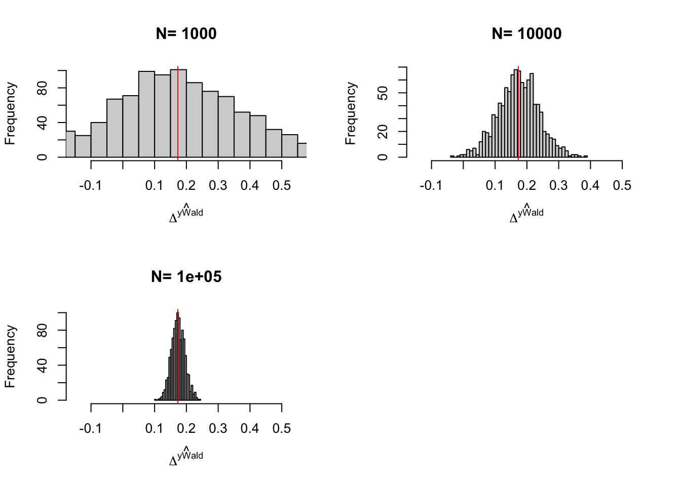
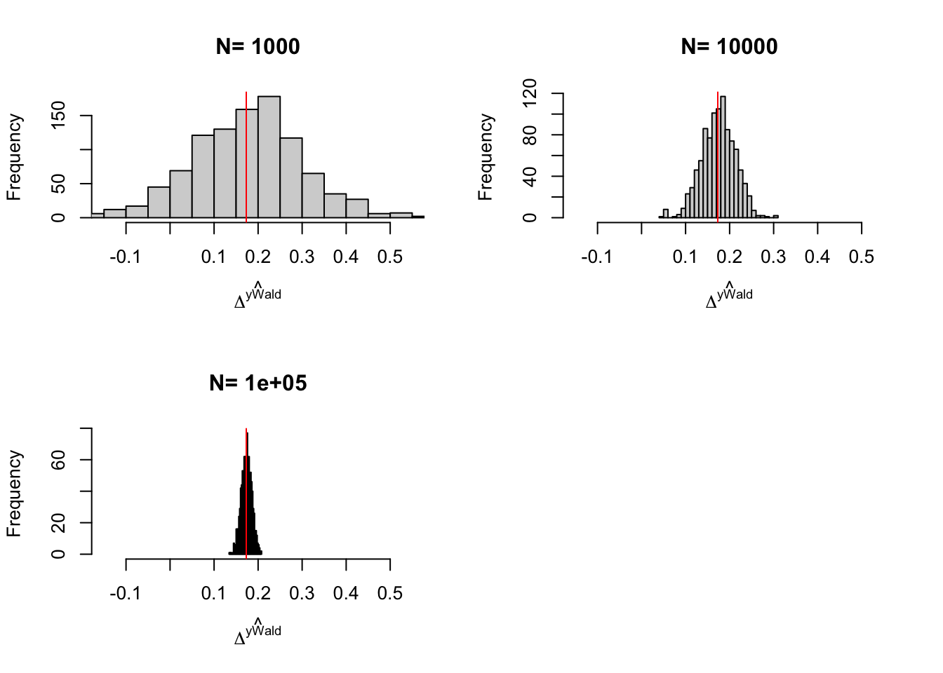
Figure 3.7: Distribution of the \(Wald\) and \(Wald(X)\) estimator in an encouragement design over replications of samples of different sizes
Comment on the results
3.4.3 Estimating sampling noise
As always, we can estimate sampling noise either using the CLT or resampling methods. Using the CLT, we can derive the following formula for the distribution of the Bloom estimator: Theorem 3.16 shows the asymptotic distribution of \(\hat{\Delta}^Y_{Wald}\):
Theorem 3.16 (Asymptotic Distribution of $\hat{\Delta}^Y_{Wald}$) Under Assumptions 3.9, 3.10, 3.11, 3.12, we have:
\[\begin{align*} \sqrt{N}(\hat{\Delta}^Y_{Wald}-\Delta^Y_{LATE}) & \stackrel{d}{\rightarrow} \mathcal{N}\left(0,\frac{1}{(p^D_1-p^D_0)^2}\left[\left(\frac{p^D}{p^R}\right)^2\frac{\var{Y_i|R_i=0}}{1-p^R}+\left(\frac{1-p^D}{1-p^R}\right)^2\frac{\var{Y_i|R_i=1}}{p^R}\right]\right)\\ \end{align*}\]
Adding Assumption 3.13, the variance of the Wald estimator can be further decomposed as follows:
\[\begin{align*} \sigma^2_{\hat{\Delta}^Y_{Wald}} & = \left(\frac{p^D}{p^R}\right)^2\frac{\var{Y_i^0|T_i=C}}{p^C(1-p^R)}+\left(\frac{1-p^D}{1-p^R}\right)^2\frac{\var{Y^1_i|T_i=C}}{p^Cp^R}\\ & \phantom{=} +\frac{(p^{AT}(1-p^R)-p^{NT}p^R)^2+p^R(1-p^R)}{(p^Cp^R(1-p^R))^2}\left[p^{AT}\var{Y_i^1|T_i=AT}+p^{NT}\var{Y^0_i|T_i=NT}\right] \end{align*}\]
with \(p^D=\Pr(D_i=1)\), \(p^R=\Pr(R_i=1)\), \(p^{D}_1=\Pr(D_i=1|R_i=1)\), \(p^{D}_0=\Pr(D_i=1|R_i=0)\), \(p^t=\Pr(T_i=t)\), with \(t\in\left\{AT,NT,C,D\right\}\).
Proof. See Section A.2.3.
Remark. Theorem 3.16 shows that the effective sample size of an encouragement design is equal to the number of compliers. Indeed, the denominator of the variance of the Wald Estimatior depends on \(p^D_1-p^D_0\), which is an estimate of the proportion of compliers, under Assumption 3.13.
Theorem 3.16 also shows that there is a price to pay for the fact that we cannot enforce the effect on always takers and never takers is actually zero. Indeed, as the second formula shows, it is not only the variance of the oucomes of the compliers that appears in the formula, but also the variances of the outcomes of the always takers and never takers, therefore increasing sampling noise.
Remark. In order to compute the formula in Theorem 3.16, we can use a plug-in estimator or the IV standard error estimate robist to heteroskedasticity. Here is a simple function in order to compute the plug-in estimator:
Example 3.31 Let us derive the CLT-based estimates of sampling noise using both the plug-in estimator and the IV standard errors without conditioning on covariates first. For the sake of the example, I’m working with a sample of size \(N=1000\).
sn.Encourag.simuls <- 2*quantile(abs(simuls.encourage[['1000']][,'Wald']-delta.y.late),probs=c(0.99))
sn.Encourag.IV.plugin <- 2*qnorm((.99+1)/2)*sqrt(var.Encourage.plugin(pD1=mean(D[E==1 & R==1]),pD0=mean(D[E==1 & R==0]),pD=mean(D[E==1]),pR=mean(R[E==1]),V0=var(y[R==0 & E==1]),V1=var(y[R==1 & E==1]),N=length(y[E==1])))
sn.Encourag.IV.homo <- 2*qnorm((.99+1)/2)*sqrt(vcov(reg.y.R.2sls.encourage)[2,2])
sn.Encourag.IV.hetero <- 2*qnorm((.99+1)/2)*sqrt(vcovHC(reg.y.R.2sls.encourage,type='HC2')[2,2])
True 99% sampling noise (from the simulations) is 1.166. 99% sampling noise estimated using the plug-in estimator is 2.124. 99% sampling noise estimated using default IV standard errors is 23.134. 99% sampling noise estimated using heteroskedasticity robust IV standard errors is 2.119.
Conditioning on \(y_i^B\):
sn.Encourag.simuls.yB <- 2*quantile(abs(simuls.encourage.yB[['1000']][,'Wald']-delta.y.late),probs=c(0.99))
sn.Encourag.IV.homo.yB <- 2*qnorm((.99+1)/2)*sqrt(vcov(reg.y.R.yB.2sls.encourage)[2,2])
sn.Encourag.IV.hetero.yB <- 2*qnorm((.99+1)/2)*sqrt(vcovHC(reg.y.R.yB.2sls.encourage,type='HC2')[2,2])
True 99% sampling noise (from the simulations) is 0.705. 99% sampling noise estimated using default IV standard errors is 0.988. 99% sampling noise estimated using heteroskedasticity robust IV standard errors is 0.975.