Chapter 2 Fundamental Problem of Statistical Inference
The Fundamental Problem of Statistical Inference (FPSI) states that, even if we have an estimator \(E\) that identifies \(TT\) in the population, we cannot observe \(E\) because we only have access to a finite sample of the population. The only thing that we can form from the sample is a sample equivalent \(\hat{E}\) to the population quantity \(E\), and \(\hat{E}\neq E\). For example, the sample analog to \(WW\) is the difference in means between treated and untreated units \(\hat{WW}\). As we saw in the last lecture, \(\hat{WW}\) is never exactly equal to \(WW\).
Why is \(\hat{E}\neq E\)? Because a finite sample is never perfectly representative of the population. In a sample, even in a random sample, the distribution of the observed and unobserved covariates deviates from the true population one. As a consequence, the sample value of the estimator is never precisely equal to the population value, but fluctuates around it with sampling noise. The main problem with the FPSI is that if we find an effect of our treatment, be it small or large, we cannot know whether we should attribute it to the treatment or to the bad or good luck of sampling noise.
What can we do to deal with the FPSI? I am going to argue that there are mainly two things that we might want to do: estimating the extent of sampling noise and decreasing sampling noise.
Estimating sampling noise means measuring how much variability there is in our estimate \(\hat{E}\) due to the sampling procedure. This is very useful because it enables us to form a confidence interval that gauges how far from \(\hat{E}\) the true value \(E\) might be. It is a measure of the precision of our estimation and of the extent to which sampling noise might drive our results. Estimating sampling noise is very hard because we have only access to one sample and we would like to know the behavior of our estimator over repeated samples. We are going to learn four ways to estimate the extent of sampling noise using data from one sample.
Because sampling noise is such a nuisance and makes our estimates imprecise, we would like to be able to make it as small as possible. We are going to study three ways of decreasing sampling noise, two that take place before collecting the data (increasing sample size, stratifying) and one that takes place after (conditioning).
Maybe you are surprised not to find statistical significance tests as an important answer to the FPSI. I argue in this lecture that statistical tests are misleading tools that make us overestimate the confidence in our results and underestimate the scope of sampling noise. Statistical tests are not meant to be used for scientific research, but were originally designed to make decisions in industrial settings where the concept of successive sampling made actual sense. Statistical tests also generate collective behaviors such as publication bias and specification search that undermine the very foundations of science. A general movement in the social sciences, but also in physics, is starting to ban the reporting of p-values.
2.1 What is sampling noise? Definition and illustration
In this section, I am going to define sampling noise and illustrate it with a numerical example. In Section 2.1.1, I define sampling noise. In section 2.1.2, I illustrate how sampling noise varies when one is interested in the population treatment effect. In section 2.1.3, I illustrate how sampling noise varies when one is interesetd in the sample treatment effect. Finally, in section 2.1.4, I show how confidence intervals can be built from an estimate of sampling noise.
2.1.1 Sampling noise, a definition
Sampling noise measures how much sampling variability moves the sample estimator \(\hat{E}\) around. One way to define it more rigorously is to make it equal to the width of a confidence interval:
Definition 2.1 (Sampling noise) Sampling noise is the width of the symmetric interval around TT within which \(\delta*100\)% of the sample estimators fall, where \(\delta\) is the confidence level. As a consequence, sampling noise is equal to \(2\epsilon\) where \(\epsilon\) is such that: \[\begin{align*} \Pr(|\hat{E}-TT|\leq\epsilon) &= \delta. \end{align*}\]
This definition tries to capture the properties of the distribution of \(\hat{E}\) using only one number. As every simplification, it leaves room for dissatisfaction, exactly as a 2D map is a convenient albeit arbitrary betrayal of a 3D phenomenon. For example, there is nothing sacred about the symmetry of the interval. It is just extremely convenient. One might prefer an interval that is symmetric in tail probabilities instead. Feel free to explore with different concepts if you like.
A related concept to that of sampling noise is that of precision: the smaller the sampling noise, the higher the precision. Precision can be defined for example as the inverse of sampling noise \(\frac{1}{2\epsilon}\).
Finally, a very useful concept is that of signal to noise ratio. It is not used in economics, but physicists use this concept all the time. The signal to noise ratio measures the treatment effect in multiple of the sampling noise. If they are of the same order of magnitude, we have a lot of noise and little confidence in our estimates. If the signal is much larger than the noise, we tend to have a lot of confidence in our parameter estimates. The signal to noise ratio can be computed as follows: \(\frac{E}{2\epsilon}\) or \(\frac{\hat{E}}{2\epsilon}\).
Remark. A very striking result is that the signal to noise ratio of a result that is marginally significant at the 5% level is very small, around one half, meaning that the noise is generally double the signal in these results. We will derive this result after studying how to estimate sampling noise with real data.
There are two distinct ways of understanding sampling noise, depending on whether we are after the population treatment effect (\(\Delta^Y_{TT}\)) or the sample treatment effect (\(\Delta^Y_{TT_s}\)). Sampling noise for the population treatment effect stems from the fact that the sample is not perfectly representative of the population. The sample differs from the population and thus the sample estimates differs from the population estimate. Sampling noise for the sample parameter stems from the fact that the control group is not a perfect embodiment of the counterfactual. Discrepancies between treated and control samples are going to generate differences between the \(WW\) estimate and the \(TT\) effect in the sample.
2.1.2 Sampling noise for the population treatment effect
Sampling noise for the population treatment effect stems from the fact that the sample is not perfectly representative of the population.
Example 2.1 In order to assess the scope of sampling noise for our population treatment effect estimate, let’s first draw a sample. In order to be able to do that, I first have to define the parameter values:
param <- c(8,.5,.28,1500,0.9,0.01,0.05,0.05,0.05,0.1)
names(param) <- c("barmu","sigma2mu","sigma2U","barY","rho","theta","sigma2epsilon","sigma2eta","delta","baralpha")
param
## barmu sigma2mu sigma2U barY rho
## 8.00 0.50 0.28 1500.00 0.90
## theta sigma2epsilon sigma2eta delta baralpha
## 0.01 0.05 0.05 0.05 0.10set.seed(1234)
N <-1000
mu <- rnorm(N,param["barmu"],sqrt(param["sigma2mu"]))
UB <- rnorm(N,0,sqrt(param["sigma2U"]))
yB <- mu + UB
YB <- exp(yB)
Ds <- rep(0,N)
V <- rnorm(N,param["barmu"],sqrt(param["sigma2mu"]+param["sigma2U"]))
Ds[V<=log(param["barY"])] <- 1
epsilon <- rnorm(N,0,sqrt(param["sigma2epsilon"]))
eta<- rnorm(N,0,sqrt(param["sigma2eta"]))
U0 <- param["rho"]*UB + epsilon
y0 <- mu + U0 + param["delta"]
alpha <- param["baralpha"]+ param["theta"]*mu + eta
y1 <- y0+alpha
Y0 <- exp(y0)
Y1 <- exp(y1)
y <- y1*Ds+y0*(1-Ds)
Y <- Y1*Ds+Y0*(1-Ds)
delta.y.ate <- function(param){
return(param["baralpha"]+param["theta"]*param["barmu"])
}In this sample, the \(WW\) estimator yields an estimate of \(\hat{\Delta^y_{WW}}=\) 0.133. Despite random assignment, we have \(\hat{\Delta^y_{WW}}\neq\Delta^y_{TT}=\) 0.18, an instance of the FPSI.
In order to see how sampling noise varies, let’s draw another sample. In order to do so, I am going to choose a different seed to initialize the pseudo-random number generator in R.
set.seed(12345)
N <-1000
mu <- rnorm(N,param["barmu"],sqrt(param["sigma2mu"]))
UB <- rnorm(N,0,sqrt(param["sigma2U"]))
yB <- mu + UB
YB <- exp(yB)
Ds <- rep(0,N)
V <- rnorm(N,param["barmu"],sqrt(param["sigma2mu"]+param["sigma2U"]))
Ds[V<=log(param["barY"])] <- 1
epsilon <- rnorm(N,0,sqrt(param["sigma2epsilon"]))
eta<- rnorm(N,0,sqrt(param["sigma2eta"]))
U0 <- param["rho"]*UB + epsilon
y0 <- mu +  U0 + param["delta"]
alpha <- param["baralpha"]+  param["theta"]*mu + eta
y1 <- y0+alpha
Y0 <- exp(y0)
Y1 <- exp(y1)
y <- y1*Ds+y0*(1-Ds)
Y <- Y1*Ds+Y0*(1-Ds)
In this sample, the \(WW\) estimator yields an estimate of \(\hat{\Delta^y_{WW}}=\) 0.179. Again, despite random assignment, we have \(\hat{\Delta^y_{WW}}\neq\Delta^y_{TT}=\) 0.18, an instance of the FPSI. Furthermore, the estimate of the population treatment effect in this sample differs from the previous one, a consequence of sampling noise.
Let’s now visualize the extent of sampling noise by repeating the procedure multiple times with various sample sizes.
This is called Monte Carlo replications: in each replication, I choose a sample size, draw one sample from the population and compute the \(\hat{WW}\) estimator.
At each replication, the sample I’m using is different, reflecting the actual sampling process and enabling me to gauge the extent of sampling noise.
In order to focus on sampling noise alone, I am running the replications in the model in which selection into the treatment is independent on potential outcomes, so that \(WW=TT\) in the population.
In order to speed up the process, I am using parallelized computing: I send each sample to a different core in my computer so that several samples can be run at the same time.
You might want to adapt the program below to the number of cores you actually have using the ncpus variable in the beginning of the .Rmd file that generates this page..
In order to parallelize computations, I use the Snowfall package in R, that gives very simple and intuitive parallelization commands.
In order to save time when generating the graph, I use the wonderful “cache” option of knitr: it stores the estimates from the code chunk and will not rerun it as long as the code inside the chunk has not been altered nor the code of the chunks that it depends on (parameter values, for example).
monte.carlo.ww <- function(s,N,param){
  set.seed(s)
  mu <- rnorm(N,param["barmu"],sqrt(param["sigma2mu"]))
  UB <- rnorm(N,0,sqrt(param["sigma2U"]))
  yB <- mu + UB
  YB <- exp(yB)
  Ds <- rep(0,N)
  V <- rnorm(N,param["barmu"],sqrt(param["sigma2mu"]+param["sigma2U"]))
  Ds[V<=log(param["barY"])] <- 1
  epsilon <- rnorm(N,0,sqrt(param["sigma2epsilon"]))
  eta<- rnorm(N,0,sqrt(param["sigma2eta"]))
  U0 <- param["rho"]*UB + epsilon
  y0 <- mu +  U0 + param["delta"]
  alpha <- param["baralpha"]+  param["theta"]*mu + eta
  y1 <- y0+alpha
  Y0 <- exp(y0)
  Y1 <- exp(y1)
  y <- y1*Ds+y0*(1-Ds)
  Y <- Y1*Ds+Y0*(1-Ds)
  return(c((1/sum(Ds))*sum(y*Ds)-(1/sum(1-Ds))*sum(y*(1-Ds)),var(y[Ds==1]),var(y[Ds==0]),mean(Ds)))
}

simuls.ww.N <- function(N,Nsim,param){
  simuls.ww <- as.data.frame(matrix(unlist(lapply(1:Nsim,monte.carlo.ww,N=N,param=param)),nrow=Nsim,ncol=4,byrow=TRUE))
  colnames(simuls.ww) <- c('WW','V1','V0','p')
  return(simuls.ww)
}

sf.simuls.ww.N <- function(N,Nsim,param){
  sfInit(parallel=TRUE,cpus=ncpus)
  sim <- as.data.frame(matrix(unlist(sfLapply(1:Nsim,monte.carlo.ww,N=N,param=param)),nrow=Nsim,ncol=4,byrow=TRUE))
  sfStop()
  colnames(sim) <- c('WW','V1','V0','p')
  return(sim)
}

simuls.ww <- lapply(N.sample,sf.simuls.ww.N,Nsim=Nsim,param=param)
## R Version: R version 4.1.1 (2021-08-10)par(mfrow=c(2,2))
for (i in 1:4){
hist(simuls.ww[[i]][,'WW'],main=paste('N=',as.character(N.sample[i])),xlab=expression(hat(Delta^yWW)),xlim=c(-0.15,0.55))
abline(v=delta.y.ate(param),col="red")
}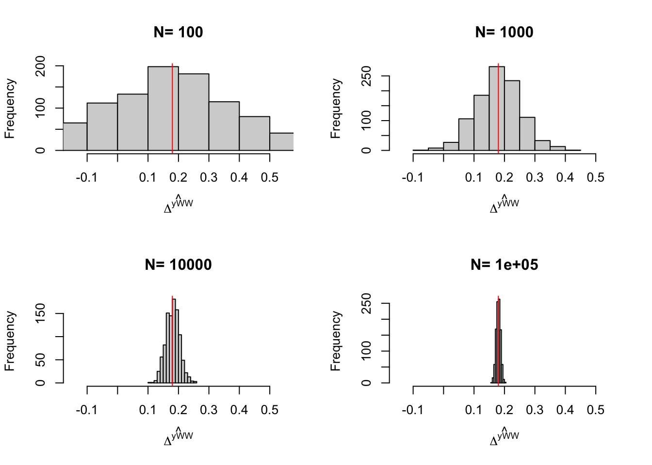
Figure 2.1: Distribution of the \(WW\) estimator over replications of samples of different sizes
Figure 2.1 is essential to understanding statistical inference and the properties of our estimators. We can see on Figure 2.1 that the estimates indeed move around at each sample replication. We can also see that the estimates seem to be concentrated around the truth. We also see that the estimates are more and more concentrated around the truth as sample size grows larger and larger.
How big is sampling noise in all of these examples? We can compute it by using the replications as approximations to the true distribution of the estimator after an infinite number of samples has been drawn. Let’s first choose a confidence level and then compute the empirical equivalent to the formula in Definition 2.1.
delta<- 0.99
delta.2 <- 0.95
samp.noise <- function(estim,delta){
  return(2*quantile(abs(delta.y.ate(param)-estim),prob=delta))
}
samp.noise.ww <- sapply(lapply(simuls.ww,`[`,,1),samp.noise,delta=delta)
names(samp.noise.ww) <- N.sample
samp.noise.ww
## 100 1000 10000 1e+05
## 1.09916429 0.39083801 0.11582492 0.03527744Let’s also compute precision and the signal to noise ratio and put all of these results together in a nice table.
precision <- function(estim,delta){
  return(1/samp.noise(estim,delta))
}
signal.to.noise <- function(estim,delta,param){
  return(delta.y.ate(param)/samp.noise(estim,delta))
}
precision.ww <- sapply(lapply(simuls.ww,`[`,,1),precision,delta=delta)
names(precision.ww) <- N.sample
signal.to.noise.ww <- sapply(lapply(simuls.ww,`[`,,1),signal.to.noise,delta=delta,param=param)
names(signal.to.noise.ww) <- N.sample
table.noise <- cbind(samp.noise.ww,precision.ww,signal.to.noise.ww)
colnames(table.noise) <- c('Sampling noise', 'Precision', 'Signal to noise ratio')
knitr::kable(table.noise,caption=paste('Sampling noise of $\\hat{WW}$ for the population treatment effect with $\\delta=$',delta,'for various sample sizes',sep=' '),booktabs=TRUE,digits = c(2,2,2),align=c('c','c','c'))| Sampling noise | Precision | Signal to noise ratio | |
|---|---|---|---|
| 100 | 1.10 | 0.91 | 0.16 |
| 1000 | 0.39 | 2.56 | 0.46 |
| 10000 | 0.12 | 8.63 | 1.55 |
| 1e+05 | 0.04 | 28.35 | 5.10 |
Finally, a nice way to summarize the extent of sampling noise is to graph how sampling noise varies around the true treatment effect, as shown on Figure 2.2.
colnames(table.noise) <- c('sampling.noise', 'precision', 'signal.to.noise')
table.noise <- as.data.frame(table.noise)
table.noise$N <- as.numeric(rownames(table.noise))
table.noise$TT <- rep(delta.y.ate(param),nrow(table.noise))
ggplot(table.noise, aes(x=as.factor(N), y=TT)) +
  geom_bar(position=position_dodge(), stat="identity", colour='black') +
  geom_errorbar(aes(ymin=TT-sampling.noise/2, ymax=TT+sampling.noise/2), width=.2,position=position_dodge(.9),color='red') +
  xlab("Sample Size")+
  theme_bw()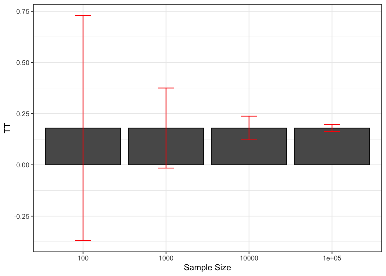
Figure 2.2: Sampling noise of \(\hat{WW}\) (99% confidence) around \(TT\) for various sample sizes
With \(N=\) 100, we can definitely see on Figure 2.2 that sampling noise is ridiculously large, especially compared with the treatment effect that we are trying to estimate. The signal to noise ratio is 0.16, which means that sampling noise is an order of magnitude bigger than the signal we are trying to extract. As a consequence, in 22.2% of our samples, we are going to estimate a negative effect of the treatment. There is also a 20.4% chance that we end up estimating an effect that is double the true effect. So how much can we trust our estimate from one sample to be close to the true effect of the treatment when \(N=\) 100? Not much.
With \(N=\) 1000, sampling noise is still large: the signal to noise ratio is 0.46, which means that sampling noise is double the signal we are trying to extract. As a consequence, the chance that we end up with a negative treatment effect has decreased to 0.9% and that we end up with an effect double the true one is 1%. But still, the chances that we end up with an effect that is smaller than three quarters of the true effect is 25.6% and the chances that we end up with an estimator that is 25% bigger than the true effect is 26.2%. These are nontrivial differences: compare a program that increases earnings by 13.5% to one that increases them by 18% and another by 22.5%. They would have completely different cost/benefit ratios. But we at least trust our estimator to give us a correct idea of the sign of the treatment effect and a vague and imprecise idea of its magnitude.
With \(N=\) 10^{4}, sampling noise is smaller than the signal, which is encouraging. The signal to noise ratio is 1.55. In only 1% of the samples does the estimated effect of the treatment become smaller than 0.125 or bigger than 0.247. We start gaining a lot of confidence in the relative magnitude of the effect, even if sampling noise is still responsible for economically significant variation.
With \(N=\) 10^{5}, sampling noise has become trivial. The signal to noise ratio is 5.1, which means that the signal is now 5 times bigger than the sampling noise. In only 1% of the samples does the estimated effect of the treatment become smaller than 0.163 or bigger than 0.198. Sampling noise is not any more responsible for economically meaningful variation.
2.1.3 Sampling noise for the sample treatment effect
Sampling noise for the sample parameter stems from the fact that the treated and control groups are not perfectly identical. The distribution of observed and unobserved covariates is actually different, because of sampling variation. This makes the actual comparison of means in the sample a noisy estimate of the true comparison that we would obtain by comparing the potential outcomes of the treated directly.
In order to understand this issue well and to be able to illustrate it correctly, I am going to focus on the average treatment effect in the whole sample, not on the treated: \(\Delta^Y_{ATE_s}=\frac{1}{N}\sum_{i=1}^N(Y_i^1-Y_i^0)\). This enables me to define a sample parameter that is independent of the allocation of \(D_i\). This is without important consequences since these two parameters are equal in the population when there is no selection bias, as we are assuming since the beginning of this lecture. Furthermore, if we view the treatment allocation generating no selection bias as a true random assignment in a Randomized Controlled Trial (RCT), then it is still possible to use this approach to estimate \(TT\) if we view the population over which we randomise as the population selected for receiving the treatment, as we will see in the lecture on RCTs.
Example 2.2 In order to assess the scope of sampling noise for our sample treatment effect estimate, we first have to draw a sample:
set.seed(1234)
N <-1000
mu <- rnorm(N,param["barmu"],sqrt(param["sigma2mu"]))
UB <- rnorm(N,0,sqrt(param["sigma2U"]))
yB <- mu + UB
YB <- exp(yB)
Ds <- rep(0,N)
V <- rnorm(N,param["barmu"],sqrt(param["sigma2mu"]+param["sigma2U"]))
Ds[V<=log(param["barY"])] <- 1
epsilon <- rnorm(N,0,sqrt(param["sigma2epsilon"]))
eta<- rnorm(N,0,sqrt(param["sigma2eta"]))
U0 <- param["rho"]*UB + epsilon
y0 <- mu +  U0 + param["delta"]
alpha <- param["baralpha"]+  param["theta"]*mu + eta
y1 <- y0+alpha
Y0 <- exp(y0)
Y1 <- exp(y1)
y <- y1*Ds+y0*(1-Ds)
Y <- Y1*Ds+Y0*(1-Ds)
In this sample, the treatment effect parameter is \(\Delta^y_{ATE_s}=\) 0.171. The \(WW\) estimator yields an estimate of \(\hat{\Delta^y_{WW}}=\) 0.133. Despite random assignment, we have \(\Delta^y_{ATE_s}\neq\hat{\Delta^y_{WW}}\), an instance of the FPSI.
In order to see how sampling noise varies, let’s draw a new treatment allocation, while retaining the same sample and the same potential outcomes.
set.seed(12345)
N <-1000
Ds <- rep(0,N)
V <- rnorm(N,param["barmu"],sqrt(param["sigma2mu"]+param["sigma2U"]))
Ds[V<=log(param["barY"])] <- 1
y <- y1*Ds+y0*(1-Ds)
Y <- Y1*Ds+Y0*(1-Ds)
In this sample, the treatment effect parameter is still \(\Delta^y_{ATE_s}=\) 0.171. The \(WW\) estimator yields now an estimate of \(\hat{\Delta^y_{WW}}=\) 0.051. The \(WW\) estimate is different from our previous estimate because the treatment was allocated to a different random subset of people.
Why is this second estimate so imprecise? It might because it estimates one of the two components of the average treatment effect badly, or both. The true average potential outcome with the treatment is, in this sample, \(\frac{1}{N}\sum_{i=1}^Ny_i^1=\) 8.207 while the \(WW\) estimate of this quantity is \(\frac{1}{\sum_{i=1}^ND_i}\sum_{i=1}^ND_iy_i=\) 8.113. The true average potential outcome without the treatment is, in this sample, \(\frac{1}{N}\sum_{i=1}^Ny_i^0=\) 8.036 while the \(WW\) estimate of this quantity is \(\frac{1}{\sum_{i=1}^N(1-D_i)}\sum_{i=1}^N(1-D_i)y_i=\) 8.062. It thus seems that most of the bias in the estimated effect stems from the fact that the treatment has been allocated to individuals with lower than expected outcomes with the treatment, be it because they did not react strongly to the treatment, or because they were in worse shape without the treatment. We can check which one of these two explanations is more important. The true average effect of the treatment is, in this sample, \(\frac{1}{N}\sum_{i=1}^N(y_i^1-y^0_i)=\) 0.171 while, in the treated group, this quantity is \(\frac{1}{\sum_{i=1}^ND_i}\sum_{i=1}^ND_i(y_i^1-y_i^0)=\) 0.18. The true average potential outcome without the treatment is, in this sample, \(\frac{1}{N}\sum_{i=1}^Ny^0_i=\) 8.036 while, in the treated group, this quantity is \(\frac{1}{\sum_{i=1}^ND_i}\sum_{i=1}^ND_iy_i^0=\) 7.933. The reason for the poor performance of the \(WW\) estimator in this sample is that individuals with lower counterfactual outcomes were included in the treated group, not that the treatment had lower effects on them. The bad counterfactual outcomes of the treated generates a bias of -0.103, while the bias due to heterogeneous reactions to the treatment is of 0.009. The last part of the bias is the one due to the fact that the individuals in the control group have slightly better counterfactual outcomes than in the sample: -0.026. The sum of these three terms yields the total bias of our \(WW\) estimator in this second sample: -0.12.
Let’s now assess the overall effect of sampling noise on the estimate of the sample treatment effect for various sample sizes. In order to do this, I am going to use parallelized Monte Carlo simulations again. For the sake of simplicity, I am going to generate the same potential outcomes in each replication, using the same seed, and only choose a different treatment allocation.
monte.carlo.ww.sample <- function(s,N,param){
  set.seed(1234)
  mu <- rnorm(N,param["barmu"],sqrt(param["sigma2mu"]))
  UB <- rnorm(N,0,sqrt(param["sigma2U"]))
  yB <- mu + UB
  YB <- exp(yB)
  epsilon <- rnorm(N,0,sqrt(param["sigma2epsilon"]))
  eta<- rnorm(N,0,sqrt(param["sigma2eta"]))
  U0 <- param["rho"]*UB + epsilon
  y0 <- mu +  U0 + param["delta"]
  alpha <- param["baralpha"]+  param["theta"]*mu + eta
  y1 <- y0+alpha
  Y0 <- exp(y0)
  Y1 <- exp(y1)
  set.seed(s)
  Ds <- rep(0,N)
  V <- rnorm(N,param["barmu"],sqrt(param["sigma2mu"]+param["sigma2U"]))
  Ds[V<=log(param["barY"])] <- 1
  y <- y1*Ds+y0*(1-Ds)
  Y <- Y1*Ds+Y0*(1-Ds)
  return((1/sum(Ds))*sum(y*Ds)-(1/sum(1-Ds))*sum(y*(1-Ds)))
}

simuls.ww.N.sample <- function(N,Nsim,param){
  return(unlist(lapply(1:Nsim,monte.carlo.ww.sample,N=N,param=param)))
}

sf.simuls.ww.N.sample <- function(N,Nsim,param){
  sfInit(parallel=TRUE,cpus=ncpus)
  sim <- sfLapply(1:Nsim,monte.carlo.ww.sample,N=N,param=param)
  sfStop()
  return(unlist(sim))
}

simuls.ww.sample <- lapply(N.sample,sf.simuls.ww.N.sample,Nsim=Nsim,param=param)

monte.carlo.ate.sample <- function(N,s,param){
  set.seed(s)
  mu <- rnorm(N,param["barmu"],sqrt(param["sigma2mu"]))
  UB <- rnorm(N,0,sqrt(param["sigma2U"]))
  yB <- mu + UB
  YB <- exp(yB)
  epsilon <- rnorm(N,0,sqrt(param["sigma2epsilon"]))
  eta<- rnorm(N,0,sqrt(param["sigma2eta"]))
  U0 <- param["rho"]*UB + epsilon
  y0 <- mu +  U0 + param["delta"]
  alpha <- param["baralpha"]+  param["theta"]*mu + eta
  y1 <- y0+alpha
  Y0 <- exp(y0)
  Y1 <- exp(y1)
  Ds <- rep(0,N)
  V <- rnorm(N,param["barmu"],sqrt(param["sigma2mu"]+param["sigma2U"]))
  Ds[V<=log(param["barY"])] <- 1
  y <- y1*Ds+y0*(1-Ds)
  Y <- Y1*Ds+Y0*(1-Ds)
  return(mean(alpha))
}

par(mfrow=c(2,2))
for (i in 1:4){
  hist(simuls.ww.sample[[i]],main=paste('N=',as.character(N.sample[i])),xlab=expression(hat(Delta^yWW)),xlim=c(-0.15,0.55))
  abline(v=monte.carlo.ate.sample(N.sample[[i]],1234,param),col="red")
}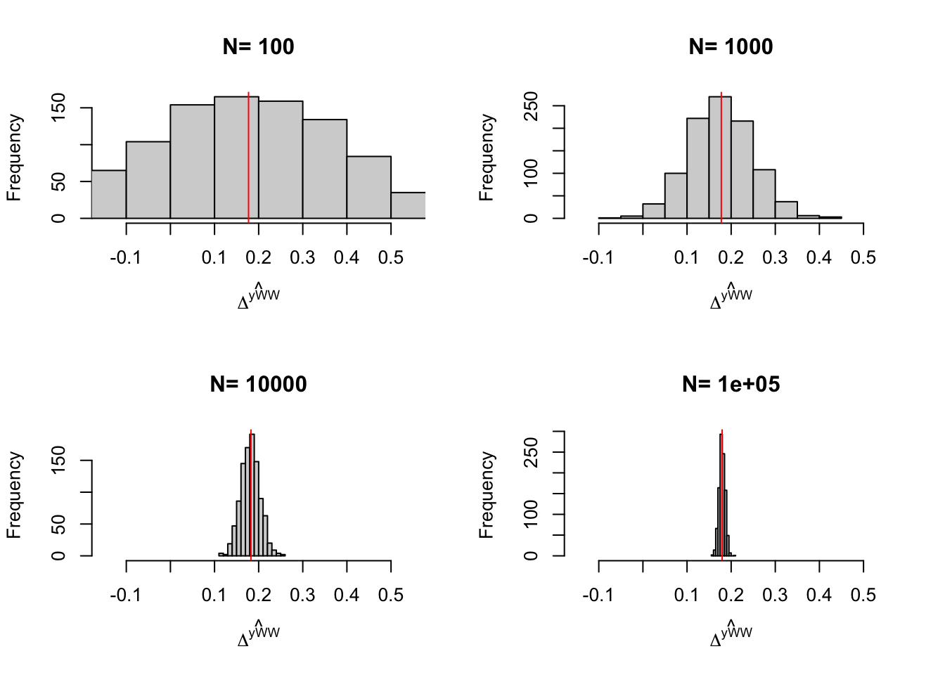
Figure 2.3: Distribution of the \(WW\) estimator over replications of treatment allocation for samples of different sizes
Let’s also compute sampling noise, precision and the signal to noise ratio in these examples.
samp.noise.sample <- function(i,delta,param){
  return(2*quantile(abs(monte.carlo.ate.sample(1234,N.sample[[i]],param)-simuls.ww.sample[[i]]),prob=delta))
}
samp.noise.ww.sample <- sapply(1:4,samp.noise.sample,delta=delta,param=param)
names(samp.noise.ww.sample) <- N.sample

precision.sample <- function(i,delta,param){
  return(1/samp.noise.sample(i,delta,param=param))
}
signal.to.noise.sample <- function(i,delta,param){
  return(monte.carlo.ate.sample(1234,N.sample[[i]],param)/samp.noise.sample(i,delta,param=param))
}
precision.ww.sample <- sapply(1:4,precision.sample,delta=delta,param=param)
names(precision.ww.sample) <- N.sample
signal.to.noise.ww.sample <- sapply(1:4,signal.to.noise.sample,delta=delta,param=param)
names(signal.to.noise.ww.sample) <- N.sample
table.noise.sample <- cbind(samp.noise.ww.sample,precision.ww.sample,signal.to.noise.ww.sample)
colnames(table.noise.sample) <- c('Sampling noise', 'Precision', 'Signal to noise ratio')
knitr::kable(table.noise.sample,caption=paste('Sampling noise of $\\hat{WW}$ for the sample treatment effect with $\\delta=$',delta,'and for various sample sizes',sep=' '),booktabs=TRUE,align=c('c','c','c'),digits=c(3,3,3))| Sampling noise | Precision | Signal to noise ratio | |
|---|---|---|---|
| 100 | 1.208 | 0.828 | 0.149 |
| 1000 | 0.366 | 2.729 | 0.482 |
| 10000 | 0.122 | 8.218 | 1.585 |
| 1e+05 | 0.033 | 30.283 | 5.453 |
Finally, let’s compare the extent of sampling noise for the population and the sample treatment effect parameters.
colnames(table.noise.sample) <- c('sampling.noise', 'precision', 'signal.to.noise')
table.noise.sample <- as.data.frame(table.noise.sample)
table.noise.sample$N <- as.numeric(rownames(table.noise.sample))
table.noise.sample$TT <- sapply(N.sample,monte.carlo.ate.sample,s=1234,param=param)
table.noise.sample$Type <- 'TTs'
table.noise$Type <- 'TT'
table.noise.tot <- rbind(table.noise,table.noise.sample)
table.noise.tot$Type <- factor(table.noise.tot$Type)

ggplot(table.noise.tot, aes(x=as.factor(N), y=TT,fill=Type)) +
  geom_bar(position=position_dodge(), stat="identity", colour='black') +
  geom_errorbar(aes(ymin=TT-sampling.noise/2, ymax=TT+sampling.noise/2), width=.2,position=position_dodge(.9),color='red') +
  xlab("Sample Size")+
  theme_bw()+
  theme(legend.position=c(0.85,0.88))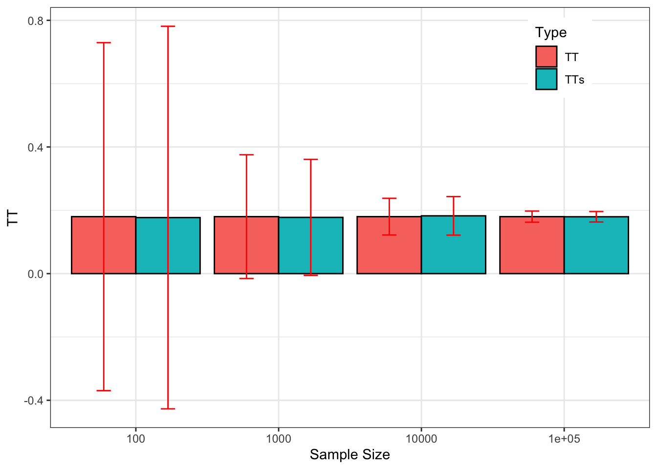
Figure 2.4: Sampling noise of \(\hat{WW}\) (99% confidence) around \(TT\) and \(TT_s\) for various sample sizes
Figure 2.3 and Table 2.2 present the results of the simulations of sampling noise for the sample treatment effect parameter.
Figure 2.4 compares sampling noise for the population and sample treatment effects.
For all practical purposes, the estimates of sampling noise for the sample treatment effect are extremely close to the ones we have estimated for the population treatment effect.
I am actually surprised by this result, since I expected that keeping the potential outcomes constant over replications would decrease sampling noise.
It seems that the variability in potential outcomes over replications of random allocations of the treatment in a given sample mimicks very well the sampling process from a population.
I do not know if this result of similarity of sampling noise for the population and sample treatment effect is a general one, but considering them as similar or close seems innocuous in our example.
2.1.4 Building confidence intervals from estimates of sampling noise
In real life, we do not observe \(TT\). We only have access to \(\hat{E}\). Let’s also assume for now that we have access to an estimate of sampling noise, \(2\epsilon\). How can we use these two quantities to assess the set of values that \(TT\) might take? One very useful device that we can use is the confidence interval. Confidence intervals are very useful because they quantify the zone within which we have a chance to find the true effect \(TT\):
Theorem 2.1 (Confidence interval) For a given level of confidence \(\delta\) and corresponding level of sampling noise \(2\epsilon\) of the estimator \(\hat{E}\) of \(TT\), the confidence interval \(\left\{\hat{E}-\epsilon,\hat{E}+\epsilon\right\}\) is such that the probability that it contains \(TT\) is equal to \(\delta\) over sample replications: \[\begin{align*} \Pr(\hat{E}-\epsilon\leq TT\leq\hat{E}+\epsilon) & = \delta. \end{align*}\]
Proof. From the definition of sampling noise, we know that: \[\begin{align*} \Pr(|\hat{E}-TT|\leq\epsilon) & = \delta. \end{align*}\] Now: \[\begin{align*} \Pr(|\hat{E}-TT|\leq\epsilon) & = \Pr(TT-\epsilon\leq\hat{E}\leq TT+\epsilon)\\ & = \Pr(-\hat{E}-\epsilon\leq-TT\leq -\hat{E}+\epsilon)\\ & = \Pr(\hat{E}-\epsilon\leq TT\leq\hat{E}+\epsilon), \end{align*}\] which proves the result.
It is very important to note that confidence intervals are centered around \(\hat{E}\) and not around \(TT\). When estimating sampling noise and building Figure 2.2, we have centered our intervals around \(TT\). The interval was fixed and \(\hat{E}\) was moving across replications and \(2\epsilon\) was defined as the length of the interval around \(TT\) containing a proportion \(\delta\) of the estimates \(\hat{E}\). A confidence interval cannot be centered around \(TT\), which is unknown, but is centered around \(\hat{E}\), that we can observe. As a consequence, it is the interval that moves around across replications, and \(\delta\) is the proportion of samples in which the interval contains \(TT\).
Example 2.3 Let’s see how confidence intervals behave in our numerical example.
N.plot <- 40
plot.list <- list()

for (k in 1:length(N.sample)){
  set.seed(1234)
  test <- sample(simuls.ww[[k]][,'WW'],N.plot)
  test <- as.data.frame(cbind(test,rep(samp.noise(simuls.ww[[k]][,'WW'],delta=delta)),rep(samp.noise(simuls.ww[[k]][,'WW'],delta=delta.2))))
  colnames(test) <- c('WW','sampling.noise.1','sampling.noise.2')
  test$id <- 1:N.plot
  plot.test <- ggplot(test, aes(x=as.factor(id), y=WW)) +
      geom_bar(position=position_dodge(), stat="identity", colour='black') +
      geom_errorbar(aes(ymin=WW-sampling.noise.1/2, ymax=WW+sampling.noise.1/2), width=.2,position=position_dodge(.9),color='red') +
      geom_errorbar(aes(ymin=WW-sampling.noise.2/2, ymax=WW+sampling.noise.2/2), width=.2,position=position_dodge(.9),color='blue') +
      geom_hline(aes(yintercept=delta.y.ate(param)), colour="#990000", linetype="dashed")+
      #ylim(-0.5,1.2)+
      xlab("Sample id")+
      theme_bw()+
      ggtitle(paste("N=",N.sample[k]))
  plot.list[[k]] <- plot.test
}
plot.CI <- plot_grid(plot.list[[1]],plot.list[[2]],plot.list[[3]],plot.list[[4]],ncol=1,nrow=length(N.sample))
print(plot.CI)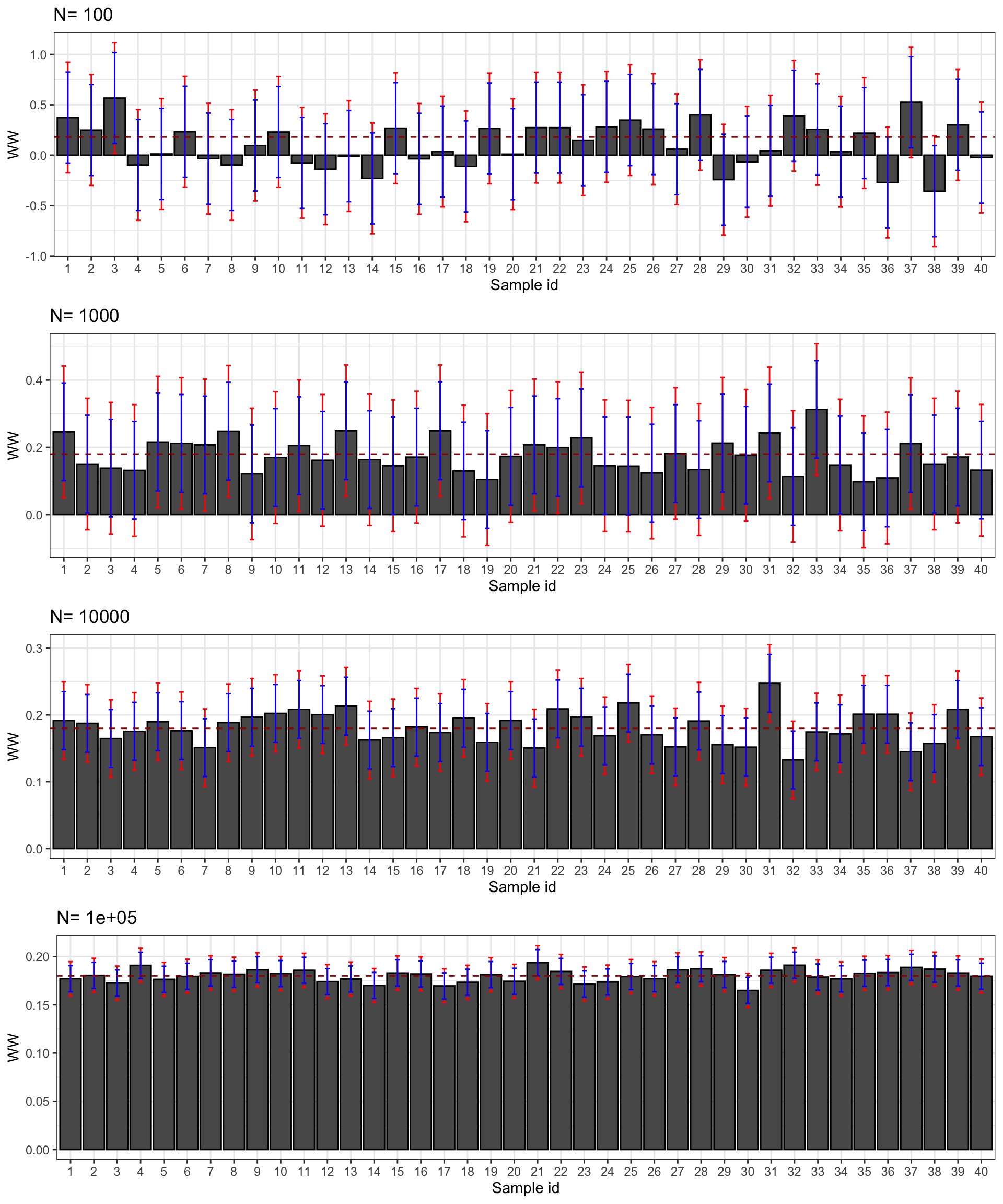
Figure 2.5: Confidence intervals of \(\hat{WW}\) for \(\delta=\) 0.99 (red) and 0.95 (blue) over sample replications for various sample sizes
Figure 2.5 presents the 99% and 95% confidence intervals for 40 samples selected from our simulations. First, confidence intervals do their job: they contain the true effect most of the time. Second, the 95% confidence interval misses the true effect more often, as expected. For example, with \(N=\) 1000, the confidence intervals in samples 13 and 23 do not contain the true effect, but it is not far from their lower bound. Third, confidence intervals faithfully reflect what we can learn from our estimates at each sample size. With \(N=\) 100, the confidence intervals make it clear that the effect might be very large or very small, even strongly negative. With \(N=\) 1000, the confidence intervals suggest that the effect is either positive or null, but unlikely to be strongly negative. Most of the time, we get the sign right. With \(N=\) 10^{4}, we know that the true effect is bigger than 0.1 and smaller than 0.3 and most intervals place the true effect somewhere between 0.11 and 0.25. With \(N=\) 10^{5}, we know that the true effect is bigger than 0.15 and smaller than 0.21 and most intervals place the true effect somewhere between 0.16 and 0.20.
2.1.5 Reporting sampling noise: a proposal
Once sampling noise is measured (and we’ll see how to get an estimate in the next section), one still has to communicate it to others. There are many ways to report sampling noise:
- Sampling noise as defined in this book (\(2*\epsilon\))
- The corresponding confidence interval
- The signal to noise ratio
- A standard error
- A significance level
- A p-value
- A t-statistic
The main problem with all of these approaches is that they do not express sampling noise in a way that is directly comparable to the magnitude of the \(TT\) estimate. Other ways of reporting sampling noise such as p-values and t-stats are nonlinear transforms of sampling noise, making it difficult to really gauge the size of sampling noise as it relates to the magnitude of \(TT\).
My own preference goes to the following format for reporting results: \(TT \pm \epsilon\). As such, we can readily compare the size of the noise to the sizee of the \(TT\) estimate. We can also form all the other ways of expressing sampling noise directly.
Example 2.4 Let’s see how this approach behaves in our numerical example.
test.all <- list()
for (k in 1:length(N.sample)){
  set.seed(1234)
  test <- sample(simuls.ww[[k]][,'WW'],N.plot)
  test <- as.data.frame(cbind(test,rep(samp.noise(simuls.ww[[k]][,'WW'],delta=delta)),rep(samp.noise(simuls.ww[[k]][,'WW'],delta=delta.2))))
  colnames(test) <- c('WW','sampling.noise.1','sampling.noise.2')
  test$id <- 1:N.plot
  test.all[[k]] <- test
}
With \(N=\) 100, the reporting of the results for sample 1 would be something like: “we find an effect of 0.37 \(\pm\) 0.55.” Note how the choice of \(\delta\) does not matter much for the result. The previous result was for \(\delta=0.99\) while the result for \(\delta=0.95\) would have been: “we find an effect of 0.37 \(\pm\) 0.45.” The precise result changes with \(\delta\), but the qualitative result stays the same: the magnitude of sampling noise is large and it dwarfs the treatment effect estimate.
With \(N=\) 1000, the reporting of the results for sample 1 with \(\delta=0.99\) would be something like: “we find an effect of 0.25 \(\pm\) 0.2.” With \(\delta=0.95\): “we find an effect of 0.25 \(\pm\) 0.15.” Again, although the precise quantitative result is affected by the choice of \(\delta\), but hte qualitative message stays the same: sampling noise is of the same order of magnitude as the estimated treatment effect.
With \(N=\) 10^{4}, the reporting of the results for sample 1 with \(\delta=0.99\) would be something like: “we find an effect of 0.19 \(\pm\) 0.06.” With \(\delta=0.95\): “we find an effect of 0.19 \(\pm\) 0.04.” Again, see how the qualitative result is independent of the precise choice of \(\delta\): sampling noise is almost one order of magnitude smaller than the treatment effect estimate.
With \(N=\) 10^{5}, the reporting of the results for sample 1 with \(\delta=0.99\) would be something like: “we find an effect of 0.18 \(\pm\) 0.02.” With \(\delta=0.95\): “we find an effect of 0.18 \(\pm\) 0.01.” Again, see how the qualitative result is independent of the precise choice of \(\delta\): sampling noise is one order of magnitude smaller than the treatment effect estimate.
Remark. What I hope the example makes clear is that my proposed way of reporting results gives the same importance to sampling noise as it gives to the treatment effect estimate. Also, comparing them is easy, without requiring a huge computational burden on our brain.
Remark. One problem with the approach that I propose is when you have a non-symetric distribution of sampling noise, or when \(TT \pm \epsilon\) exceeds natural bounds on \(TT\) (such as if the effect cannot be bigger than one, for example). I think these issues are minor and rare and can be dealt with on a case by case basis. The advantage of having one simple and directly readable number comparable to the magnitude of the treatment effect is overwhelming and makes this approach the most natural and adequate, in my opinion.
2.1.6 Using effect sizes to normalize the reporting of treatment effects and their precision
When looking at the effect of a program on an outcome, we depend on the scaling on that outcome to appreciate the relative size of the estimated treatment effect.
It is often difficult to appreciate the relative importance of the size of an effect, even if we know the scale of the outcome of interest.
One useful device to normalize the treatment effects is called Cohen’s \(d\), or effect size.
The idea is to compare the magnitude of the treatment effect to an estimate of the usual amount of variation that the outcome undergoes in the population.
The way to build Cohen’s \(d\) is by dividing the estimated treatment effect by the standard deviation of the outcome.
I generally prefer to use the standard devaition of the outcome in the control group, so as not to include the additional amoiunt of variation due to the heterogeneity in treatment effects.
Definition 2.2 (Cohen's $d$) Cohen’s \(d\), or effect size, is the ratio of the estimated treatment effect to the standard deviation of outcomes in the control group:
\[ d = \frac{\hat{TT}}{\sqrt{\frac{1}{N^0}\sum_{i=1}^{N^0}(Y_i-\bar{Y^0})^2}} \] where \(\hat{TT}\) is an estimate of the treatment effect, \(N^0\) is the number of individuals in the treatment group and \(\bar{Y^0}\) is the average outcome in the treatment group.
Cohen’s \(d\) can be interpreted in terms of magnitude of effect size:
- It is generally considered that an effect is large when its \(d\) is larger than 0.8.
- An effect size around 0.5 is considered medium
- An effect size around 0.2 is considered to be small
- An effect size around 0.02 is considered to be very small.
There probably could be a rescaling of these terms, but that is the actual state of the art.
What I like about effect sizes is that they encourage an interpretation of the order of magnitude of the treatment effect. As such, they enable to include the information on precision by looking at which orders of magnitude are compatible with the estimated effect at the estimated precision level. Effect sizes and orders of magnitude help make us aware that our results might be imprecise, and that the precise value that we have estimated is probably not the truth. What is important is the range of effect sizes compatible with our results (both point estimate and precision).
Example 2.5 Let’s see how Cohen’s \(d\) behaves in our numerical example.
The value of Cohen’s \(d\) (or effect size) in the population is equal to:
\[\begin{align*} ES & = \frac{TT}{\sqrt{V^0}} = \frac{\bar{\alpha}+\theta\bar{\mu}}{\sqrt{\sigma^2_{\mu}+\rho^2\sigma^2_{U}+\sigma^2_{\epsilon}}} \end{align*}\]
We can write a function to compute this parameter, as well as functions to implement its estimator in the simulated samples:
V0 <- function(param){
  return(param["sigma2mu"]+param["rho"]^2*param["sigma2U"]+param["sigma2epsilon"])
}

ES <- function(param){
  return(delta.y.ate(param)/sqrt(V0(param)))
}

samp.noise.ES <- function(estim,delta,param=param){
  return(2*quantile(abs(delta.y.ate(param)/sqrt(V0(param))-estim),prob=delta))
}

for (i in 1:4){
  simuls.ww[[i]][,'ES'] <- simuls.ww[[i]][,'WW']/sqrt(simuls.ww[[i]][,'V0'])
}
The true effect size in the population is thus 0.2. It is considered to be small according to the current classification, although I’d say that a treatment able to move the outcomes by 20% of their usual variation is a pretty effective treatment, and this effect should be labelled at least medium. Let’s stick with the classification though. In our example, the effect size does not differ much from the treatment effect since the standard deviation of outcomes in the control group is pretty close to one: it is equal to 0.88. Let’s now build confidence intervals for the effect size and try to comment on the magnitudes of these effects using the normalized classification.
N.plot.ES <- 40
plot.list.ES <- list()

for (k in 1:length(N.sample)){
  set.seed(1234)
  test.ES <- sample(simuls.ww[[k]][,'ES'],N.plot)
  test.ES <- as.data.frame(cbind(test.ES,rep(samp.noise.ES(simuls.ww[[k]][,'ES'],delta=delta,param=param)),rep(samp.noise.ES(simuls.ww[[k]][,'ES'],delta=delta.2,param=param))))
  colnames(test.ES) <- c('ES','sampling.noise.ES.1','sampling.noise.ES.2')
  test.ES$id <- 1:N.plot.ES
  plot.test.ES <- ggplot(test.ES, aes(x=as.factor(id), y=ES)) +
      geom_bar(position=position_dodge(), stat="identity", colour='black') +
      geom_errorbar(aes(ymin=ES-sampling.noise.ES.1/2, ymax=ES+sampling.noise.ES.1/2), width=.2,position=position_dodge(.9),color='red') +
      geom_errorbar(aes(ymin=ES-sampling.noise.ES.2/2, ymax=ES+sampling.noise.ES.2/2), width=.2,position=position_dodge(.9),color='blue') +
      geom_hline(aes(yintercept=ES(param)), colour="#990000", linetype="dashed")+
      #ylim(-0.5,1.2)+
      xlab("Sample id")+
      ylab("Effect Size")+
      theme_bw()+
      ggtitle(paste("N=",N.sample[k]))
  plot.list.ES[[k]] <- plot.test.ES
}
plot.CI.ES <- plot_grid(plot.list.ES[[1]],plot.list.ES[[2]],plot.list.ES[[3]],plot.list.ES[[4]],ncol=1,nrow=length(N.sample))
print(plot.CI.ES)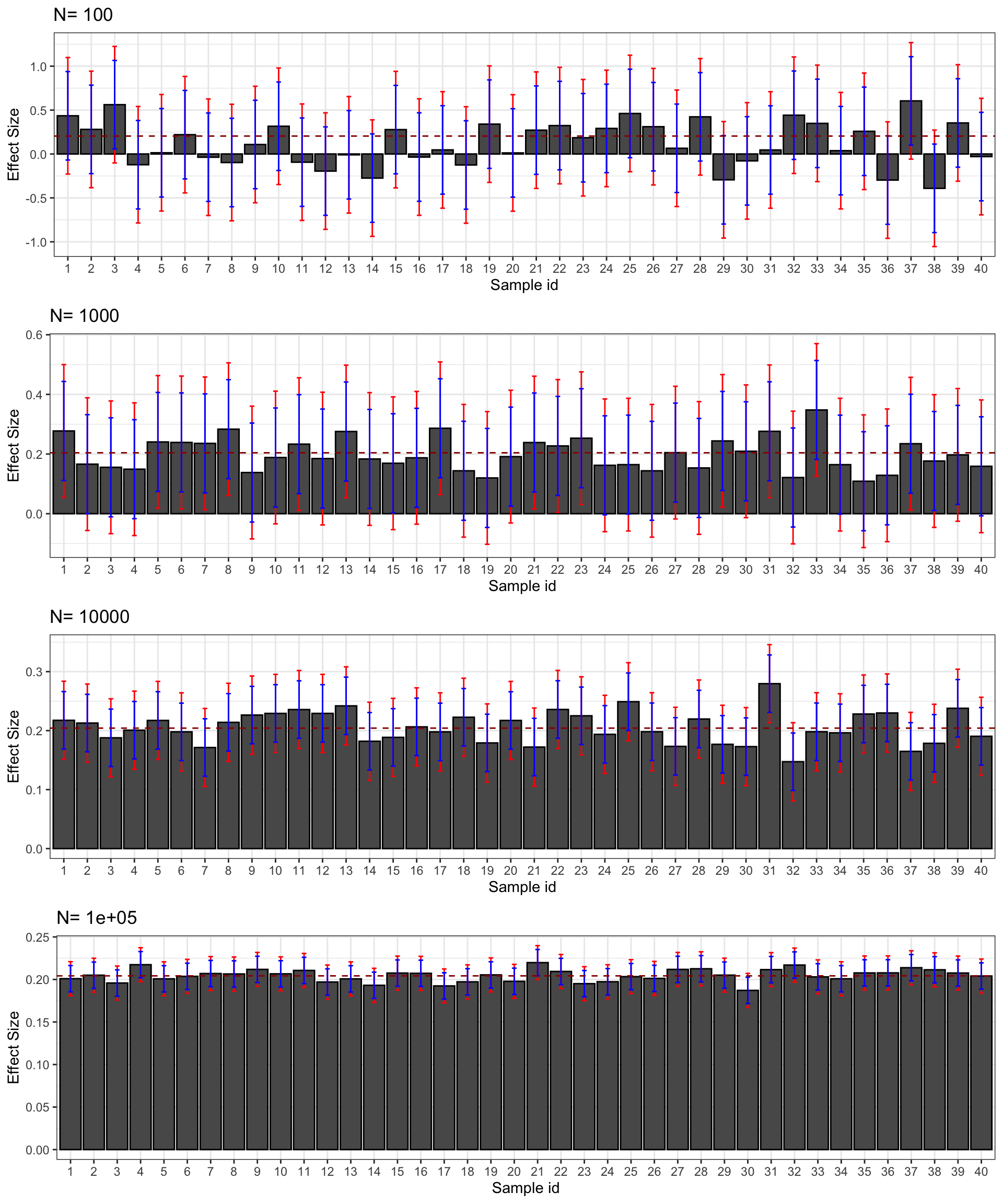
Figure 2.6: Confidence intervals of \(\hat{ES}\) for \(\delta=\) 0.99 (red) and 0.95 (blue) over sample replications for various sample sizes
Figure 2.6 presents the 99% and 95% confidence intervals for the effect size estimated in 40 samples selected from our simulations. Let’s regroup our estimate and see how we could present their results.
test.all.ES <- list()
for (k in 1:length(N.sample)){
  set.seed(1234)
  test.ES <- sample(simuls.ww[[k]][,'ES'],N.plot)
  test.ES <- as.data.frame(cbind(test.ES,rep(samp.noise.ES(simuls.ww[[k]][,'ES'],delta=delta,param=param)),rep(samp.noise.ES(simuls.ww[[k]][,'ES'],delta=delta.2,param=param))))
  colnames(test.ES) <- c('ES','sampling.noise.ES.1','sampling.noise.ES.2')
  test.ES$id <- 1:N.plot.ES
  test.all.ES[[k]] <- test.ES
}
With \(N=\) 100, the reporting of the results for sample 1 would be something like: “we find an effect size of 0.44 \(\pm\) 0.66” with \(\delta=0,99\). With \(\delta=0.95\) we would say: “we find an effect of 0.44 \(\pm\) 0.5.” All in all, our estimate is compatible with the treatment having a large positive effect size and a medium negative effect size. Low precision prevents us from saying much else.
With \(N=\) 1000, the reporting of the results for sample 1 with \(\delta=0.99\) would be something like: “we find an effect size of 0.28 \(\pm\) 0.22.” With \(\delta=0.95\): “we find an effect size of 0.28 \(\pm\) 0.17.” Our estimate is compatible with a medium positive effect or a very small positive or even negative effect (depending on the choice of \(\delta\)).
With \(N=\) 10^{4}, the reporting of the results for sample 1 with \(\delta=0.99\) would be something like: “we find an effect size of 0.22 \(\pm\) 0.07.” With \(\delta=0.95\): “we find an effect size of 0.22 \(\pm\) 0.05.” Our estimate is thus compatible with a small effect of the treatment. We can rule out that the effect of the treatment is medium since the upper bound of the 99% confidence interval is equal to 0.28. We can also rule out that the effect of the treatment is very small since the lower bound of the 99% confidence interval is equal to 0.15. With this sample size, we have been able to reach a precision level sufficient enough to pin down the order of magnitude of the effect size of our treatment. There still remains a considerable amount of uncertainty about the true effect size, though: the upper bound of our confidence interval is almost double the lower bound.
With \(N=\) 10^{5}, the reporting of the results for sample 1 with \(\delta=0.99\) would be something like: “we find an effect size of 0.2 \(\pm\) 0.02.” With \(\delta=0.95\): “we find an effect size of 0.2 \(\pm\) 0.02.” Here, the level of precision of our result is such that, first, it does not depend on the choice of \(\delta\) in any meaningful way, and second, we can do more than pinpoint the order of magnitude of the effect size, we can start to zero in on its precise value. From our estimate, the true value of the effect size is really close to 0.2. It could be equal to 0.18 or 0.22, but not further away from 0.2 than that. Remember that is actually equal to 0.2.
Remark. One issue with Cohen’s \(d\) is that its magnitude depends on the dispersion of the outcomes in the control group. That means that for the same treatment, and same value of the treatment effect, the effect size is larger in a population where oucomes are more homogeneous. This is not an attractive feature of a normalizing scale that its size depends on the particular application. One solution would be, for each outcome, to provide a standardized scale, using for example the estmated standard deviation in a reference population. This would be similar to the invention of the metric system, where a reference scale was agreed uppon once and for all.
Remark. Cohen’s \(d\) is well defined for continuous outcomes. For discrete outcomes, the use of Cohen’s \(d\) poses a series of problems, and alternatives such as relative risk ratios and odds ratios have been proposed. I’ll comment on that in the last chapter.
2.2 Estimating sampling noise
Gauging the extent sampling noise is very useful in order to be able to determine how much we should trust our results. Are they precise, so that the true treatment effect lies very close to our estimate? Or are our results imprecise, the true treatment effect maybe lying very far from our estimate?
Estimating sampling noise is hard because we want to infer a property of our estimator over repeated samples using only one sample. In this lecture, I am going to introduce four tools that enable you to gauge sampling noise and to choose sample size. The four tools are Chebyshev’s inequality, the Central Limit Theorem, resampling methods and Fisher’s permutation method. The idea of all these methods is to use the properties of the sample to infer the properties of our estimator over replications. Chebyshev’s inequality gives an upper bound on the sampling noise and a lower bound on sample size, but these bounds are generally too wide to be useful. The Central Limit Theorem (CLT) approximates the distribution of \(\hat{E}\) by a normal distribution, and quantifies sampling noise as a multiple of the standard deviation. Resampling methods use the sample as a population and draw new samples from it in order to approximate sampling noise. Fisher’s permutation method, also called randomization inference, derives the distribution of \(\hat{E}\) under the assumption that all treatment effects are null, by reallocating the treatment indicator among the treatment and control group. Both the CLT and resampling methods are approximation methods, and their approximation of the true extent of sampling noise gets better and better as sample size increases. Fisher’s permutation method is exact-it is not an approximation-but it only works for the special case of the \(WW\) estimator in a randomized design.
The remaining of this section is structured as follows. Section 2.2.1 introduces the assumptions that we will need in order to implement the methods. Section 2.2.2 presents the Chebyshev approach to gauging sampling noise and choosing sample size. Section 2.2.3 introduces the CLT way of approximating sampling noise and choosing sample size. Section 2.2.4 presents the resampling methods.
Remark. I am going to derive the estimators for the precision only for the \(WW\) estimator. In the following lectures, I will show how these methods adapt to other estimators.
2.2.1 Assumptions
In order to be able to use the theorems that power up the methods that we are going to use to gauge sampling noise, we need to make some assumptions on the properties of the data. The main assumptions that we need are that the estimator identifies the true effect of the treatment in the population, that the estimator is well-defined in the sample, that the observations in the sample are independently and identically distributed (i.i.d.), that there is no interaction between units and that the variances of the outcomes in the treated and untreated group are finite.
We know from last lecture that for the \(WW\) estimator to identify \(TT\), we need to assume that there is no selection bias, as stated in Assumption 1.7. One way to ensure that this assumption holds is to use a RCT.
In order to be able to form the \(WW\) estimator in the sample, we also need that there is at least one treated and one untreated in the sample:
Hypothesis 2.1 (Full rank) We assume that there is at least one observation in the sample that receives the treatment and one observation that does not receive it: \[\begin{align*} \exists i,j\leq N \text{ such that } & D_i=1 \& D_j=0. \end{align*}\]
One way to ensure that this assumption holds is to sample treated and untreated units.
In order to be able to estimate the variance of the estimator easily, we assume that the observations come from random sampling and are i.i.d.:
Hypothesis 2.2 (i.i.d. sampling) We assume that the observations in the sample are identically and independently distributed: \[\begin{align*} \forall i,j\leq N\text{, }i\neq j\text{, } & (Y_i,D_i)\Ind(Y_j,D_j),\\ & (Y_i,D_i)\&(Y_j,D_j)\sim F_{Y,D}. \end{align*}\]
We have to assume something on how the observations are related to each other and to the population. Identical sampling is natural in the sense that we are OK to assume that the observations stem from the same population model. Independent sampling is something else altogether. Independence means that the fates of two closely related individuals are assumed to be independent. This rules out two empirically relevant scenarios:
- The fates of individuals are related because of common influences, as for example the environment, etc,
- The fates of individuals are related because they directly influence each other, as for example on a market, but also for example because there are diffusion effects, such as contagion of deseases or technological adoption by imitation.
We will address both sources of failure of the independence assumption in future lectures.
Finally, in order for all our derivations to make sense, we need to assume that the outcomes in both groups have finite variances, otherwise sampling noise is going to be too extreme to be able to estimate it using the methods developed in this lecture:
Hypothesis 2.3 (Finite variance of potential outcomes) We assume that \(\var{Y^1|D_i=1}\) and \(\var{Y^0|D_i=0}\) are finite.
2.2.2 Using Chebyshev’s inequality
Chebyshev’s inequality is a fundamental building block of statistics. It relates the sampling noise of an estimator to its variance. More precisely, it derives an upper bound on the samplig noise of an unbiased estimator:
Theorem 2.2 (Chebyshev's inequality) For any unbiased estimator \(\hat{\theta}\), sampling noise level \(2\epsilon\) and confidence level \(\delta\), sampling noise is bounded from above:
\[\begin{align*} 2\epsilon \leq 2\sqrt{\frac{\var{\hat{\theta}}}{1-\delta}}. \end{align*}\]
Remark. The more general version of Chebyshev’s inequality that is generally presented is as follows:
\[\begin{align*} \Pr(|\hat{\theta}-\esp{\hat{\theta}}|>\epsilon) & \leq \frac{\var{\hat{\theta}}}{\epsilon^2}. \end{align*}\]
The version I present in Theorem 2.2 is adapted to the bouding of sampling noise for a given confidence level, while this version is adapted to bounding the confidence level for a given level of sampling noise. In order to go from this general version to Theorem 2.2, simply remember that, for an unbiased estimator, \(\esp{\hat{\theta}}=\theta\) and that, by definition of sampling noise, \(\Pr(|\hat{\theta}-\theta|>\epsilon)=1-\delta\). As a result, \(1-\delta\leq\var{\hat{\theta}}/\epsilon^2\), hence the result in Theorem 2.2.
Using Chebyshev’s inequality, we can obtain an upper bound on the sampling noise of the \(WW\) estimator:
Theorem 2.3 (Upper bound on the sampling noise of $\hat{WW}$) Under Assumptions 1.7, 2.1 and 2.2, for a given confidence level \(\delta\), the sampling noise of the \(\hat{WW}\) estimator is bounded from above:
\[\begin{align*} 2\epsilon \leq 2\sqrt{\frac{1}{N(1-\delta)}\left(\frac{\var{Y_i^1|D_i=1}}{\Pr(D_i=1)}+\frac{\var{Y_i^0|D_i=0}}{1-\Pr(D_i=1)}\right)}\equiv 2\bar{\epsilon}. \end{align*}\]
Proof. See in Appendix A.1.1
Theorem 2.3 is a useful step forward for estimating sampling noise. Theorem 2.3 states that the actual level of sampling noise of the \(\hat{WW}\) estimator (\(2\epsilon\)) is never bigger than a quantity that depends on sample size, confidence level and on the variances of outcomes in the treated and control groups. We either know all the components of the formula for \(2\bar{\epsilon}\) or we can estimate them in the sample. For example, \(\Pr(D_i=1)\), \(\var{Y_i^1|D_i=1}\) and \(\var{Y_i^0|D_i=0}\) by can be approximated by, respectively:
\[\begin{align*} \hat{\Pr(D_i=1)} & = \frac{1}{N}\sum_{i=1}^ND_i\\ \hat{\var{Y_i^1|D_i=1}} & = \frac{1}{\sum_{i=1}^ND_i}\sum_{i=1}^ND_i(Y_i-\frac{1}{\sum_{i=1}^ND_i}\sum_{i=1}^ND_iY_i)^2\\ \hat{\var{Y_i^0|D_i=0}} & = \frac{1}{\sum_{i=1}^N(1-D_i)}\sum_{i=1}^N(1-D_i)(Y_i-\frac{1}{\sum_{i=1}^N(1-D_i)}\sum_{i=1}^N(1-D_i)Y_i)^2. \end{align*}\]
Using these approximations for the quantities in the formula, we can compute an estimate of the upper bound on sampling noise, \(\hat{2\bar{\epsilon}}\).
Example 2.6 Let’s write an R function that is going to compute an estimate for the upper bound of sampling noise for any sample:
Let’s estimate this upper bound in our usual sample:
set.seed(1234)
N <-1000
delta <- 0.99
mu <- rnorm(N,param["barmu"],sqrt(param["sigma2mu"]))
UB <- rnorm(N,0,sqrt(param["sigma2U"]))
yB <- mu + UB
YB <- exp(yB)
Ds <- rep(0,N)
V <- rnorm(N,param["barmu"],sqrt(param["sigma2mu"]+param["sigma2U"]))
Ds[V<=log(param["barY"])] <- 1
epsilon <- rnorm(N,0,sqrt(param["sigma2epsilon"]))
eta<- rnorm(N,0,sqrt(param["sigma2eta"]))
U0 <- param["rho"]*UB + epsilon
y0 <- mu +  U0 + param["delta"]
alpha <- param["baralpha"]+  param["theta"]*mu + eta
y1 <- y0+alpha
Y0 <- exp(y0)
Y1 <- exp(y1)
y <- y1*Ds+y0*(1-Ds)
Y <- Y1*Ds+Y0*(1-Ds)
In our sample, for \(\delta=\) 0.99, \(\hat{2\bar{\epsilon}}=\) 1.35. How does this compare with the true extent of sampling noise when \(N=\) 1000? Remember that we have computed an estimate of sampling noise out of our Monte Carlo replications. In Table 2.2, we can read that sampling noise is actually equal to 0.39. The Chebyshev upper bound overestimates the extent of sampling noise by 245%.
How does the Chebyshev upper bound fares overall? In order to know that, let’s compute the Chebyshev upper bound for all the simulated samples. You might have noticed that, when running the Monte Carlo simulations for the population parameter, I have not only recovered \(\hat{WW}\) for each sample, but also the estimates of the components of the formula for the upper bound on sampling noise. I can thus easily compute the Chebyshev upper bound on sampling noise for each replication.
for (k in (1:length(N.sample))){
  simuls.ww[[k]]$cheb.noise <- samp.noise.ww.cheb(N.sample[[k]],delta,simuls.ww[[k]][,'V1'],simuls.ww[[k]][,'V0'],simuls.ww[[k]][,'p'])
}
par(mfrow=c(2,2))
for (i in 1:4){
  hist(simuls.ww[[i]][,'cheb.noise'],main=paste('N=',as.character(N.sample[i])),xlab=expression(hat(2*bar(epsilon))),xlim=c(0.25*min(simuls.ww[[i]][,'cheb.noise']),max(simuls.ww[[i]][,'cheb.noise'])))
  abline(v=table.noise[i,colnames(table.noise)=='sampling.noise'],col="red")
}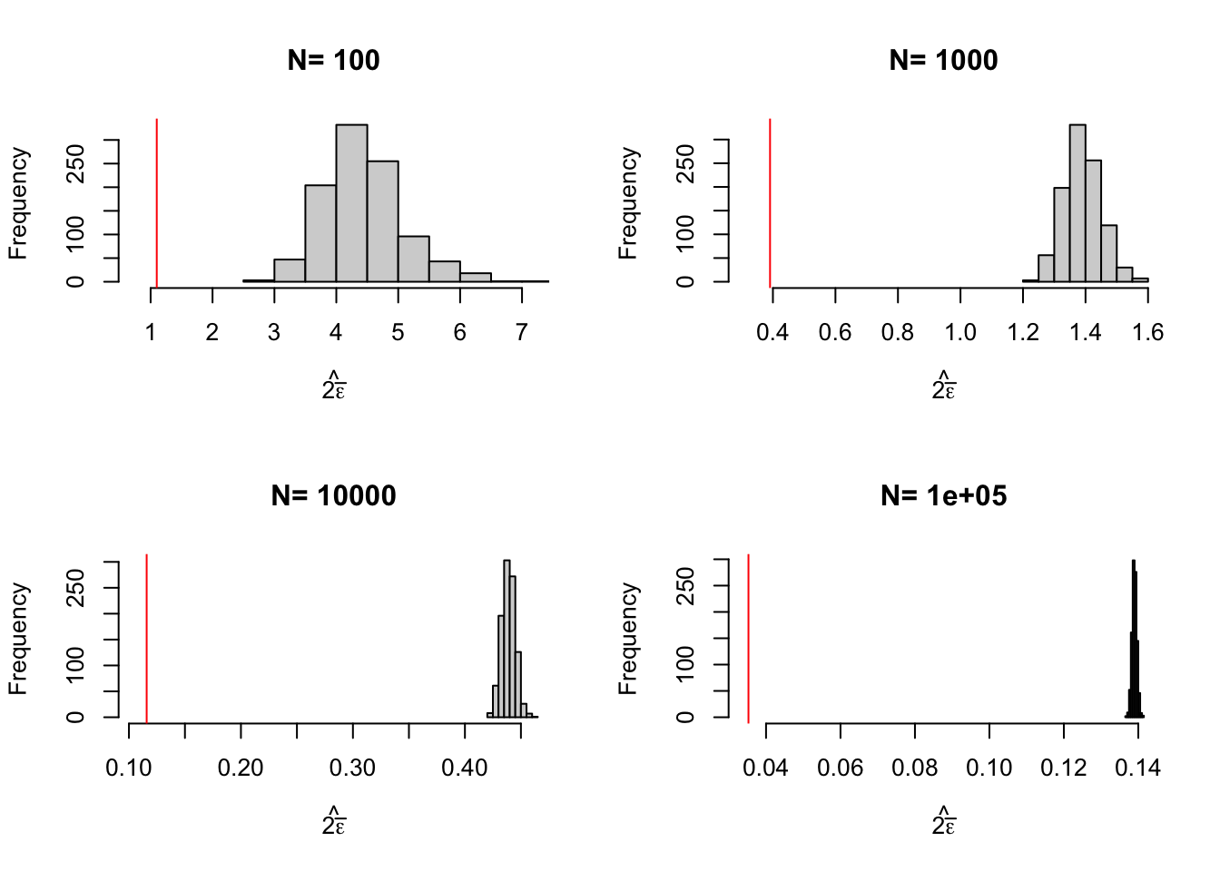
Figure 2.7: Distribution of the Chebyshev upper bound on sampling noise over replications of samples of different sizes (true sampling noise in red)
Figure 2.7 shows that the upper bound works: it is always bigger than the true sampling noise. Figure 2.7 also shows that the upper bound is large: it generally is of an order of magnitude bigger than the true sampling noise, and thus offers a blurry and too pessimistic view of the precision of an estimator. Figure 2.8 shows that the average Chebyshev bound gives an inflated estimate of sampling noise. Figure 2.9 shows that the Chebyshev confidence intervals are clearly less precise than the true unknown ones. With \(N=\) 1000, the true confidence intervals generally reject large negative effects, whereas the Chebyshev confidence intervals do not rule out this possibility. With \(N=\) 10^{4}, the true confidence intervals generally reject effects smaller than 0.1, whereas the Chebyshev confidence intervals cannot rule out small negative effects.
As a conclusion on Chebyshev estimates of sampling noise, their advantage is that they offer an upper bound on the noise: we can never underestimate noise if we use them. A downside of Chebyshev sampling noise estimates is their low precision, which makes it hard to pinpoint the true confidence intervals.
for (k in (1:length(N.sample))){
  table.noise$cheb.noise[k] <- mean(simuls.ww[[k]]$cheb.noise)
}
ggplot(table.noise, aes(x=as.factor(N), y=TT)) +
  geom_bar(position=position_dodge(), stat="identity", colour='black') +
  geom_errorbar(aes(ymin=TT-sampling.noise/2, ymax=TT+sampling.noise/2), width=.2,position=position_dodge(.9),color='red') +
  geom_errorbar(aes(ymin=TT-cheb.noise/2, ymax=TT+cheb.noise/2), width=.2,position=position_dodge(.9),color='blue') +
  xlab("Sample Size")+
  theme_bw()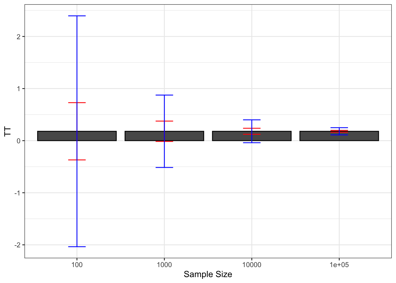
Figure 2.8: Average Chebyshev upper bound on sampling noise over replications of samples of different sizes (true sampling noise in red)
N.plot <- 40
plot.list <- list()

for (k in 1:length(N.sample)){
  set.seed(1234)
  test.cheb <- simuls.ww[[k]][sample(N.plot),c('WW','cheb.noise')]
  test.cheb <- as.data.frame(cbind(test.cheb,rep(samp.noise(simuls.ww[[k]][,'WW'],delta=delta),N.plot)))
  colnames(test.cheb) <- c('WW','cheb.noise','sampling.noise')
  test.cheb$id <- 1:N.plot
  plot.test.cheb <- ggplot(test.cheb, aes(x=as.factor(id), y=WW)) +
      geom_bar(position=position_dodge(), stat="identity", colour='black') +
      geom_errorbar(aes(ymin=WW-sampling.noise/2, ymax=WW+sampling.noise/2), width=.2,position=position_dodge(.9),color='red') +
      geom_errorbar(aes(ymin=WW-cheb.noise/2, ymax=WW+cheb.noise/2), width=.2,position=position_dodge(.9),color='blue') +
      geom_hline(aes(yintercept=delta.y.ate(param)), colour="#990000", linetype="dashed")+
      xlab("Sample id")+
      theme_bw()+
      ggtitle(paste("N=",N.sample[k]))
  plot.list[[k]] <- plot.test.cheb
}
plot.CI <- plot_grid(plot.list[[1]],plot.list[[2]],plot.list[[3]],plot.list[[4]],ncol=1,nrow=length(N.sample))
print(plot.CI)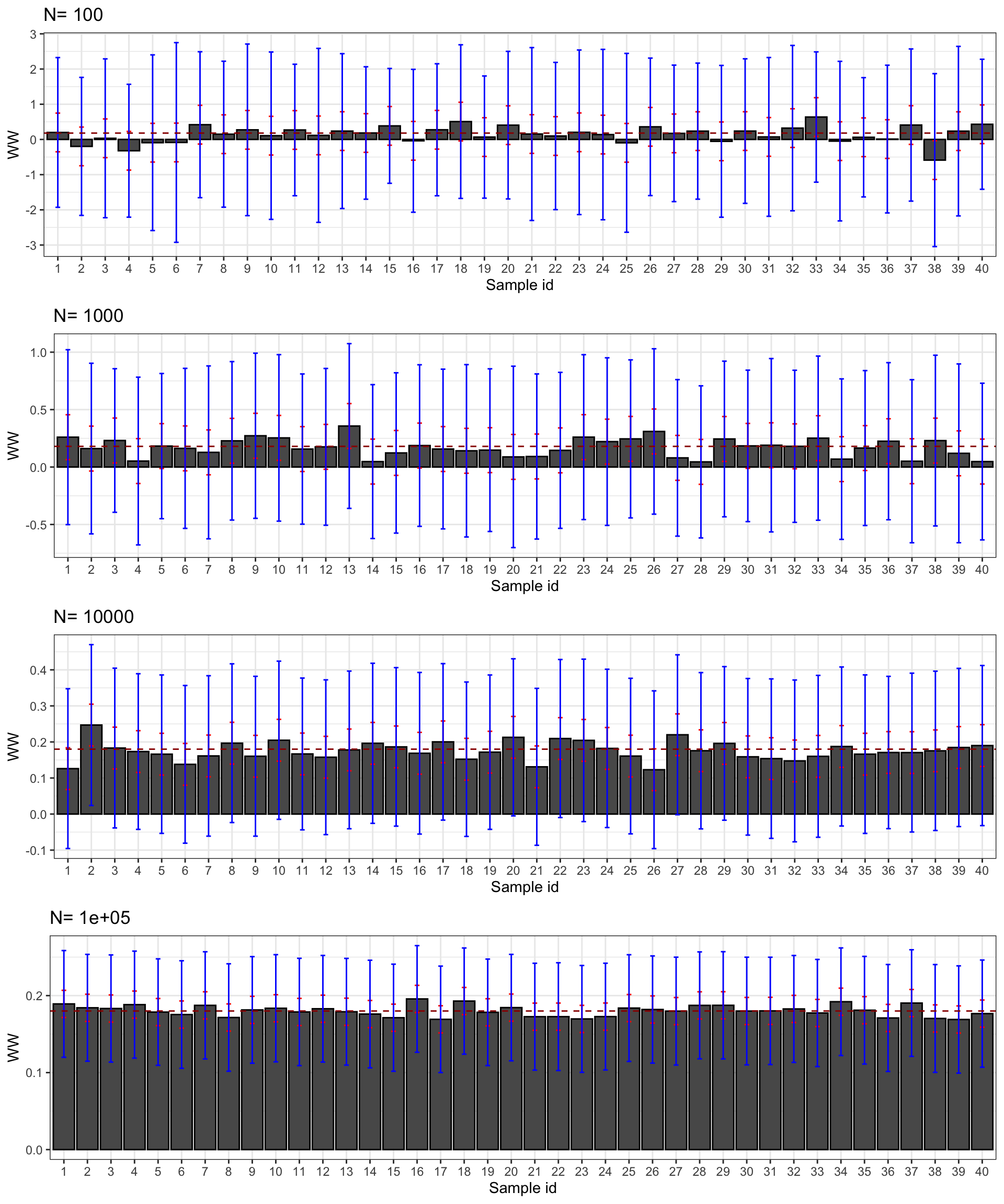
Figure 2.9: Chebyshev confidence intervals of \(\hat{WW}\) for \(\delta=\) 0.99 over sample replications for various sample sizes (true confidence intervals in red)
2.2.3 Using the Central Limit Theorem
The main problem with Chebyshev’s upper bound on sampling noise is that it is an upper bound, and thus it overestimates sampling noise and underestimates precision. One alternative to using Chebyshev’s upper bound is to use the Central Limit Theorem (CLT). In econometrics and statistics, the CLT is used to derive approximate values for the sampling noise of estimators. Because these approximations become more and more precise as sample size increases, we call them asymptotic approximations.
Taken to its bare bones, the CLT states that the sum of i.i.d. random variables behaves approximately like a normal distribution when the sample size is large:
Theorem 2.4 (Central Limit Theorem) Let \(X_i\) be i.i.d. random variables with \(\esp{X_i}=\mu\) and \(\var{X_i}=\sigma^2\), and define \(Z_N=\frac{\frac{1}{N}\sum_{i=1}^NX_i-\mu}{\frac{\sigma}{\sqrt{N}}}\), then, for all \(z\) we have:
\[\begin{align*} \lim_{N\rightarrow\infty}\Pr(Z_N\leq z) & = \Phi(z), \end{align*}\] where \(\Phi\) is the cumulative distribution function of the centered standardized normal.
We say that \(Z_N\) converges in distribution to a standard normal random variable, and we denote: \(Z_N\stackrel{d}{\rightarrow}\mathcal{N}(0,1)\).
The CLT is a beautiful result: the distribution of the average of realisations of any random variable that has finite mean and variance can be approximated by a normal when the sample size is large enough. The CLT is somehow limited though because not all estimators are sums. Estimators are generally more or less complex combinations of sums. In order to derive the asymptotic approximation for a lot of estimators that are combinations of sums, econometricians and statisticians complement the CLT with two other extremely powerful tools: Slutsky’s theorem and the Delta method. Slutsky’s theorem states that sums, products and ratios of sums that converge to a normal converge to the sum, product or ratio of these normals. The Delta method states that a function of a sum that converges to a normal converges to a normal whose variance is a quadratic form of the variance of the sum and of the first derivative of the function. Both of these tools are stated more rigorously in the appendix, but you do not need to know them for this class. The idea is for you to be aware of how the main approximations that we are going to use throughout this class have been derived.
Let me now state the main result of this section:
Theorem 2.5 (Asymptotic Estimate of Sampling Noise of WW) Under Assumptions 1.7, 2.1, 2.2 and 2.3, for a given confidence level \(\delta\) and sample size \(N\), the sampling noise of \(\hat{WW}\) can be approximated as follows:
\[\begin{align*} 2\epsilon & \approx 2\Phi^{-1}\left(\frac{\delta+1}{2}\right)\frac{1}{\sqrt{N}}\sqrt{\frac{\var{Y_i^1|D_i=1}}{\Pr(D_i=1)}+\frac{\var{Y_i^0|D_i=0}}{1-\Pr(D_i=1)}} \equiv 2\tilde{\epsilon}. \end{align*}\]
Proof. See in Appendix A.1.2.
Let’s write an R function that computes this formula:
samp.noise.ww.CLT <- function(N,delta,v1,v0,p){
  return(2*qnorm((delta+1)/2)*sqrt((v1/p+v0/(1-p))/N))
}
Example 2.7 Let’s see how the CLT performs in our example.
In our sample, for \(\delta=\) 0.99, the CLT estimate of sampling noise is \(\hat{2\tilde{\epsilon}}=\) 0.35. How does this compare with the true extent of sampling noise when \(N=\) 1000? Remember that we have computed an estimate of sampling noise out of our Monte Carlo replications. In Table 2.1, we can read that sampling noise is actually equal to 0.39. The CLT approximation is pretty precise: it only underestimates the true extent of sampling noise by 11%.
We can also compute the CLT approximation to sampling noise in all of our samples:
for (k in (1:length(N.sample))){
  simuls.ww[[k]]$CLT.noise <- samp.noise.ww.CLT(N.sample[[k]],delta,simuls.ww[[k]][,'V1'],simuls.ww[[k]][,'V0'],simuls.ww[[k]][,'p'])
}
par(mfrow=c(2,2))
for (i in 1:4){
  hist(simuls.ww[[i]][,'CLT.noise'],main=paste('N=',as.character(N.sample[i])),xlab=expression(hat(2*bar(epsilon))),xlim=c(min(simuls.ww[[i]][,'CLT.noise']),max(simuls.ww[[i]][,'CLT.noise'])))
  abline(v=table.noise[i,colnames(table.noise)=='sampling.noise'],col="red")
}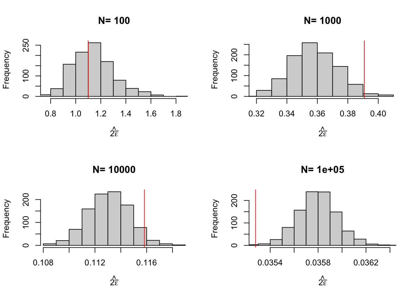
Figure 2.10: Distribution of the CLT approximation of sampling noise over replications of samples of different sizes (true sampling noise in red)
Figure 2.10 shows that the CLT works: CLT-based estimates of sampling noise approximates true sampling noise well. CLT-based approximations of sampling noise are even impressively accurate: they always capture the exact order of magnitude of sampling noise, although there is a slight underestimation when \(N=\) 1000 and 10^{4} and a slight overestimation when \(N=\) 10^{5}. This success should not come as a surprise as all shocks in our model are normally distributed, meaning that the CLT results are more than an approximation, they are exact. Results might be less spectacular when estimating the effect of the treatment on the outcomes in levels rather than in logs.
As a consequence, the average CLT-based estimates of sampling noise and of confidence intervals are pretty precise, as Figures 2.11 and 2.12 show. Let’s pause for a second at the beauty of what we have achieved using the CLT: by using only information from one sample, we have been able to gauge extremely precisely how the estimator would behave over sampling repetitions.
for (k in (1:length(N.sample))){
  table.noise$CLT.noise[k] <- mean(simuls.ww[[k]]$CLT.noise)
}
ggplot(table.noise, aes(x=as.factor(N), y=TT)) +
  geom_bar(position=position_dodge(), stat="identity", colour='black') +
  geom_errorbar(aes(ymin=TT-sampling.noise/2, ymax=TT+sampling.noise/2), width=.2,position=position_dodge(.9),color='red') +
  geom_errorbar(aes(ymin=TT-CLT.noise/2, ymax=TT+CLT.noise/2), width=.2,position=position_dodge(.9),color='blue') +
  xlab("Sample Size")+
  theme_bw()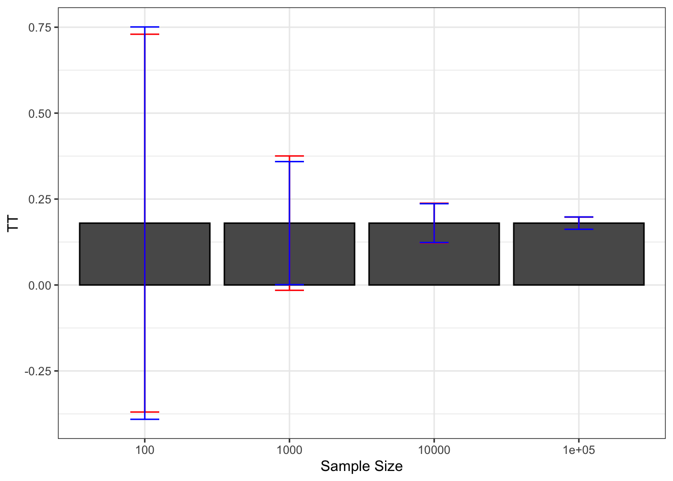
Figure 2.11: Average CLT-based approximations of sampling noise over replications of samples of different sizes (true sampling noise in red)
N.plot <- 40
plot.list <- list()

for (k in 1:length(N.sample)){
  set.seed(1234)
  test.CLT <- simuls.ww[[k]][sample(N.plot),c('WW','CLT.noise')]
  test.CLT <- as.data.frame(cbind(test.CLT,rep(samp.noise(simuls.ww[[k]][,'WW'],delta=delta),N.plot)))
  colnames(test.CLT) <- c('WW','CLT.noise','sampling.noise')
  test.CLT$id <- 1:N.plot
  plot.test.CLT <- ggplot(test.CLT, aes(x=as.factor(id), y=WW)) +
      geom_bar(position=position_dodge(), stat="identity", colour='black') +
      geom_errorbar(aes(ymin=WW-sampling.noise/2, ymax=WW+sampling.noise/2), width=.2,position=position_dodge(.9),color='red') +
      geom_errorbar(aes(ymin=WW-CLT.noise/2, ymax=WW+CLT.noise/2), width=.2,position=position_dodge(.9),color='blue') +
      geom_hline(aes(yintercept=delta.y.ate(param)), colour="#990000", linetype="dashed")+
      xlab("Sample id")+
      theme_bw()+
      ggtitle(paste("N=",N.sample[k]))
  plot.list[[k]] <- plot.test.CLT
}
plot.CI <- plot_grid(plot.list[[1]],plot.list[[2]],plot.list[[3]],plot.list[[4]],ncol=1,nrow=length(N.sample))
print(plot.CI)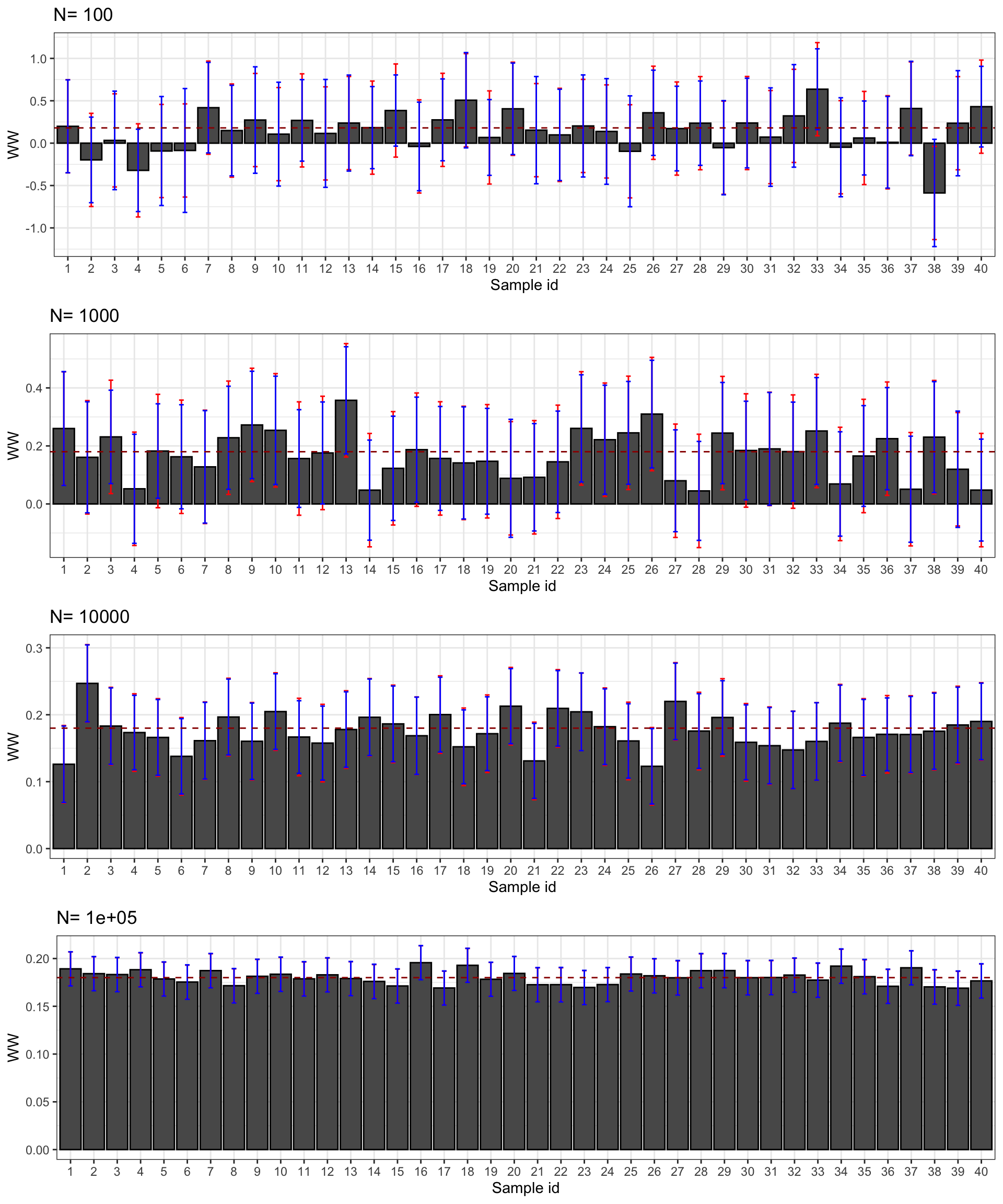
Figure 2.12: CLT-based confidence intervals of \(\hat{WW}\) for \(\delta=\) 0.99 over sample replications for various sample sizes (true confidence intervals in red)
Remark. In proving the main result on the asymptotic distribution of \(\hat{WW}\), we have also proved a very useful result: \(\hat{WW}\) is the Ordinary Least Squares (OLS) estimator of \(\beta\) in the regression \(Y_i=\alpha+\beta D_i + U_i\). This is pretty cool since we now can use our classical OLS estimator in our statistical package to estimate \(\hat{WW}\). Let’s compute the OLS estimate of \(WW\) in our sample:
We have \(\hat{WW}_{OLS}=\) 0.13 \(=\) 0.13 \(=\hat{WW}\).
Remark. Another pretty cool consequence of Theorem 2.5 and of its proof is that the standard error of the OLS estimator of \(\hat{WW}\) (\(\sigma_{\beta}\)) is related to the sampling noise of \(\hat{WW}\) by the following formula: \(2\tilde{\epsilon}=2\Phi^{-1}\left(\frac{\delta+1}{2}\right)\sigma_{\beta}\).
This implies that sampling noise is equal to 5 \(\sigma_{\beta}\) when \(\delta=\) 0.99 and to 4 \(\sigma_{\beta}\) when \(\delta=\) 0.95. It is thus very easy to move from estimates of the standard error of the \(\beta\) coefficient to the extent of sampling noise.
Remark. A last important consequence of Theorem 2.5 and of its proof is that the standard error of the OLS estimator of \(\hat{WW}\) (\(\sigma_{\beta}\)) that we use is the heteroskedasticity-robust one.
Using the RCM, we can indeed show that:
\[\begin{align*} \alpha & = \esp{Y_i^0|D_i=0} \\ \beta & = \Delta^Y_{TT} \\ U_i & = Y^0_i-\esp{Y^0_i|D_i=0} + D_i(\Delta^Y_i-\Delta^Y_{TT}), \end{align*}\]
Under Assumption 1.7, we have:
\[\begin{align*} U_i & = (1-D_i)(Y^0_i-\esp{Y^0_i|D_i=0}) + D_i(Y_i^1-\esp{Y^1_i|D_i=1}) \end{align*}\]
There is heteroskedasticity because the outcomes of the treated and of the untreated have different variances:
\[\begin{align*} \var{U_i|D_i=d} & = \esp{U_i^2|D_i=d} \\ & = \esp{(Y^d_i-\esp{Y^d_i|D_i=d})^2|D_i=d} \\ & = \var{Y_i^d|D_i=d} \end{align*}\]
We do not want to assume homoskedasticity, since it would imply a constant treatment effect. Indeed, \(\var{Y_i^1|D_i=1} = \var{Y_i^0|D_i=1}+\var{\alpha_i|D_i=1}\).
Remark. In order to estimate the heteroskedasticity robust standard error from the OLS regression, we can use the sandwich package in R Most available heteroskedasticity robust estimators based on the CLT can be written in the following way:
\[\begin{align*} \var{\hat{\Theta}_{OLS}} & \approx (X'X)^{-1}X'\hat{\Omega}X(X'X)^{-1}, \end{align*}\]
where \(X\) is the matrix of regressors and \(\hat{\Omega}=\diag(\hat{\sigma}^2_{U_1},\dots,\hat{\sigma}^2_{U_N})\) is an estimate the covariance matrix of the residuals \(U_i\). Here are various classical estimators for \(\hat{\Omega}\):
\[\begin{align*} \text{HC0:} & & \hat{\sigma_{U_i}}^2 & = \hat{U_i}^2 \\ \text{HC1:} & & \hat{\sigma_{U_i}}^2 & = \frac{N}{N-K}\hat{U_i}^2 \\ \text{HC2:} & & \hat{\sigma_{U_i}}^2 & = \frac{\hat{U_i}^2}{1-h_i} \\ \text{HC3:} & & \hat{\sigma_{U_i}}^2 & = \frac{\hat{U_i}^2}{(1-h_i)^2}, \end{align*}\]
where \(\hat{U}_i\) is the residual from the OLS regression, \(K\) is the number of regressors, \(h_i\) is the leverage of observation \(i\), and is the \(i^{\text{th}}\) diagonal element of \(H=X(X'X)^{-1}X'\). HC1 is the one reported by Stata when using the ‘robust’ option.
Example 2.8 Using the sandwich package, we can estimate the heteroskedasticity-robust variance-covariance matrix and sampling noise as follows:
ols.ww.vcov.HC0 <- vcovHC(ols.ww, type = "HC0")
samp.noise.ww.CLT.ols <- function(delta,reg,...){
  return(2*qnorm((delta+1)/2)*sqrt(vcovHC(reg,...)[2,2]))
}
For \(\delta=\) 0.99, sampling noise estimated using the “HC0” option is equal to 0.35. This is exactly the value we have estimated using our CLT-based formula (\(\hat{2\tilde{\epsilon}}=\) 0.35). Remember that sampling noise is actually equal to 0.39. Other “HC” options might be better in small samples. For example, with the “HC1” option, we have an estimate for sampling noise of 0.35. What would have happened to our estimate of sampling noise if we had ignored heteroskedasticity? The default OLS standard error estimate yields an estimate for sampling noise of 0.36.
2.2.4 Using resampling methods
The main intuition behind resampling methods is to use the sample as a population, to draw samples from it and compute our estimator on each of these samples in order to gauge its variability over sampling repetitions. There are three main methods of resampling that work that way: bootstrapping, radomization inference and subsampling. Bootstrapping draws samples with replacement, so that each sample has the same size as the original sample. Subsampling draws samples without replacement, thereby the samples are of a smaller size than the original one. Randomization inference keeps the same sample in all repetitions, but changes the allocation of the treatment.
Why would we use resampling methods instead of CLT-based standard errors? There are several possible reasons:
- Asymptotic refinements: sometimes, resampling methods are more precise in small samples than the CLT-based asymptotic approaches. In that case, we say that resampling methods offer asymptotic refinements.
- Ease of computation: for some estimators, the CLT-based estimates of sampling noise are complex or cumbersome to compute, whereas resampling methods are only computationally intensive.
- Inexistence of CLT-based estimates of sampling noise: some estimators do not have any CLT-based estimates of sampling noise yet. That was the case for the Nearest-Neighbour Matching estimator (NNM) for a long time for example. It still is the case for the Synthetic Control Method estimator. Beware though that the bootstrap is not valid for all estimators. For example, it is possible to show that the bootstrap is invalid for NNM. Subsampling is valid for NNM though (see Abadie and Imbens, 2006).
2.2.4.1 Bootstrap
The basic idea of the bootstrap is to use Monte Carlo replications to draw samples from the original sample with replacement. Then, at each replication, we compute the value of our estimator \(\hat{E}\) on the new sample. Let’s call this new value \(\hat{E}^*_k\) for bootstrap replication \(k\). Under certain conditions, the distribution of \(\hat{E}^*_k\) approximates the distribution of \(\hat{E}\) over sample repetitions very well, and all the more so as the sample size gets large.
What are the conditions under which the bootstrap is going to provide an accurate estimation of the distribution of \(\hat{E}\)? Horowitz (2001) reports on a very nice result by Mammen that makes these conditions clear:
Theorem 2.6 (Mammen (1992)) Let \(\left\{X_i:i=1,\dots,N\right\}\) be a random sample from a population. For a sequence of functions \(g_N\) and sequences of numbers \(t_N\) and \(\sigma_N\), define \(\bar{g}_N=\frac{1}{N}\sum_{i=1}^Ng_N(X_i)\) and \(T_N=(\bar{g}_N-t_N)/\sigma_N\). For the bootstrap sample \(\left\{X^*_i:i=1,\dots,N\right\}\), define \(\bar{g}^*_N=\frac{1}{N}\sum_{i=1}^Ng_N(X^*_i)\) and \(T^*_N=(\bar{g}^*_N-\bar{g}_N)/\sigma_N\). Let \(G_N(\tau)=\Pr(T_N\leq\tau)\) and \(G^*_N(\tau)=\Pr(T^*_N\leq\tau)\), where this last probability distribution is taken over bootstrap sampling replications. Then \(G^*_N\) consistently estimates \(G_N\) if and only if \(T_N\stackrel{d}{\rightarrow}\mathcal{N}(0,1)\).
Theorem 2.6 states that the bootstrap will offer a consistent estimation of the distribution of a given estimator if and only if this estimator is asymptotically normally distributed. It means that we could theoretically use the CLT-based asymptotic distribution to compute sampling noise. So, and it demands to be stronlgy emphasized, .
How do we estimate sampling noise with the bootstrap? There are several ways to do so, but I am going to emphasize the most widespread here, that is known as the percentile method. Let’s define \(E^*_{\frac{1-\delta}{2}}\) and \(E^*_{\frac{1+\delta}{2}}\) as the corresponding quantiles of the bootstrap distribution of \(\hat{E}^*_k\) over a large number \(K\) of replications. The bootstrapped sampling noise using the percentile method is simply the distance between these two quantities.
Theorem 2.7 (Bootstrapped Estimate of Sampling Noise of WW) Under Assumptions 1.7, 2.1, 2.2 and 2.3, for a given confidence level \(\delta\) and sample size \(N\), the sampling noise of \(\hat{WW}\) can be approximated as follows:
\[\begin{align*} 2\epsilon & \approx E^*_{\frac{1+\delta}{2}}-E^*_{\frac{1-\delta}{2}} \equiv 2\tilde{\epsilon}^b. \end{align*}\]
Proof. The \(WW\) estimator can be written as a sum:
\[\begin{align*} \hat{\Delta^Y_{WW}} & = \frac{1}{N}\sum_{i=1}^N\frac{\left(Y_i-\frac{1}{N}\sum_{i=1}^NY_i\right)\left(D_i-\frac{1}{N}\sum_{i=1}^ND_i\right)}{\frac{1}{N}\sum_{i=1}^N\left(D_i-\frac{1}{N}\sum_{i=1}^ND_i\right)^2}. \end{align*}\]
Using Lemma A.5, we know that the \(WW\) estimator is asymptotically normal under Assumptions 1.7, ??, 2.2 and ??. Using Theorem 2.6 proves the result.
Remark. With the bootstrap, we are not going to define the confidence interval using Theorem 2.1 but directly using \(\left\{E^*_{\frac{1-\delta}{2}};E^*_{\frac{1+\delta}{2}}\right\}\). Indeed, we have defined the bootstrapped estimator of sampling noise by using the asymetric confidence interval. We could have used the equivalent of Definition 2.1 on the bootstrapped samples to compute sampling noise using the symmetric confidence interval. Both are feasible and similar in large samples, since the asymptotic distribution is symmetric. One advantage of asymetric confidence intervals is that they might capture deviations from the normal distribution in small samples. These advantages are part of what we call asymptotic refinements. Rigorously, though, asymptotic refinements have not been proved to exist for the percentile method but only for the method bootstrapping asymptotically pivotal quantities.
Remark. We say that a method brings asymptotic refinements if it increases the precision when estimating sampling noise and confidence intervals relative to the asymptotic CLT-based approximation. The bootstrap has been shown rigorously to bring asymptotic refinements when used to estimate the distribution of asymptotically pivotal statistic. An asymptotically pivotal statistic is a statistic that can be computed from the sample but that, asymptotically, converges to a quantity that does not depend on the sample, like for example a standard normal. Using Lemma A.5, we know for example that the following statistic is asymptotically normal:
\[\begin{align*} T_N^{WW} & = \frac{\hat{\Delta^Y_{WW}}-\Delta^Y_{TT}}{\sqrt{\frac{\frac{\var{Y_i^1|D_i=1}}{\Pr(D_i=1)}+\frac{\var{Y_i^0|D_i=0}}{1-\Pr(D_i=1)}}{N}}} \stackrel{d}{\rightarrow}\mathcal{N}\left(0,1\right). \end{align*}\]
To build a confidence interval bootstrapping \(T_N^{WW}\), compute an estimator of \(T_N^{WW}\) for each bootstrapped sample, say \(\hat{T}_{N,k}^{WW*}\). You can for example use the OLS estimator in the bootstrapped sample, with a heteroskedasticity-robust standard error estimator. Or you can compute the \(WW\) estimator by hand in the sample along with an estimator of its variance using the variance of the outcomes in the treated and control groups. You can then estimate the confidence interval as follows: \(\left\{\hat{\Delta^Y_{WW}}-\hat{\sigma_{WW}}\hat{T}^{WW*}_{N,\frac{1-\delta}{2}};\hat{\Delta^Y_{WW}}+\hat{\sigma_{WW}}\hat{T}^{WW*}_{N,\frac{1+\delta}{2}}\right\}\), where \(\hat{T}^{WW*}_{N,q}\) iq the \(q^{\text{th}}\) quantile of the distribution of \(\hat{T}_{N,k}^{WW*}\) over sampling replications and \(\hat{\sigma_{WW}}\) is an estimate of the variance of \(\hat{\Delta^Y_{WW}}\) (either the CLT-based approximation of the bootstrapped one, see below).
Remark. One last possibility to develop an estimator for sampling noise and confidence interval is to use the bootstrap in order to estimate the variance of the estimator \(\hat{E}\), \(\hat{\sigma^2_{E}}\), and then use it to compute sampling noise. If \(\hat{E}\) is asymptotically normally distributed, we have that sampling noise is equal to \(2\Phi^{-1}\left(\frac{\delta+1}{2}\right)\hat{\sigma_{E}}\). You can use the usual formula from Theore 2.1 to compute the confidence interval. The bootstrapped variance of \(\hat{E}\), \(\hat{\sigma^2_{E}}\), is simply the variance of \(\hat{E}^*_k\) over bootstrap replications.
Example 2.9 In the numerical example, I am going to derive the bootstrapped confidence intervals and sampling noise for the percentile method. Let’s first put the dataset from our example in a nice data frame format so that resampling is made easier. We then define a function taking a number of bootstrapped replications and spitting out sampling noise and confidence intervals.
data <- as.data.frame(cbind(y,Ds,yB))
boot.fun.ww.1 <- function(seed,data){
  set.seed(seed,kind="Wichmann-Hill")
  data <- data[sample(nrow(data),replace = TRUE),]
  ols.ww <- lm(y~Ds,data=data)
  ww <- ols.ww$coef[[2]]
  return(ww)
}

boot.fun.ww <- function(Nboot,data){
  #sfInit(parallel=TRUE,cpus=8)
  boot <- lapply(1:Nboot,boot.fun.ww.1,data=data)
  #sfStop()
  return(unlist(boot))
}

boot.CI.ww <- function(boot,delta){
  return(c(quantile(boot,prob=(1-delta)/2),quantile(boot,prob=(1+delta)/2)))
}

boot.samp.noise.ww <- function(boot,delta){
  return(quantile(boot,prob=(1+delta)/2)-quantile(boot,prob=(1-delta)/2))
}

Nboot <- 500
ww.boot <- boot.fun.ww(Nboot,data)
ww.CI.boot <- boot.CI.ww(ww.boot,delta)
ww.samp.noise.boot <- boot.samp.noise.ww(ww.boot,delta)
Over 500 replications, the 99% bootstrapped confidence interval using the percentile method is \(\left\{-0.027;0.295\right\}\). As a consequence, the bootstrapped estimate of 99% sampling noise is of 0.321. Remember that, with \(N=\) 1000, sampling noise is actually equal to 0.39.
In order to assess the global precision of bootstrapping, we are going to resort to Monte Carlo simulations. For each Monte Carlo sample, we are going to estimate sampling noise and confidence intervals using the bootstrap. As you can imagine, this is going to prove rather computationally intensive. I cannot use parallelization twice: I have to choose whether to parallelize the Monte Carlo simulations or the bootstrap simulations. I have choosen to parallelize the outer loop, so that a given job takes longer on each cluster.
monte.carlo.ww.boot <- function(s,N,param,Nboot,delta){
  set.seed(s)
  mu <- rnorm(N,param["barmu"],sqrt(param["sigma2mu"]))
  UB <- rnorm(N,0,sqrt(param["sigma2U"]))
  yB <- mu + UB
  YB <- exp(yB)
  Ds <- rep(0,N)
  V <- rnorm(N,param["barmu"],sqrt(param["sigma2mu"]+param["sigma2U"]))
  Ds[V<=log(param["barY"])] <- 1
  epsilon <- rnorm(N,0,sqrt(param["sigma2epsilon"]))
  eta<- rnorm(N,0,sqrt(param["sigma2eta"]))
  U0 <- param["rho"]*UB + epsilon
  y0 <- mu +  U0 + param["delta"]
  alpha <- param["baralpha"]+  param["theta"]*mu + eta
  y1 <- y0+alpha
  Y0 <- exp(y0)
  Y1 <- exp(y1)
  y <- y1*Ds+y0*(1-Ds)
  Y <- Y1*Ds+Y0*(1-Ds)
  data <- as.data.frame(cbind(y,Ds,yB))
  ww.boot <- boot.fun.ww(Nboot,data)
  ww.CI.boot <- boot.CI.ww(ww.boot,delta)
  ww.samp.noise.boot <- boot.samp.noise.ww(ww.boot,delta)
  return(c((1/sum(Ds))*sum(y*Ds)-(1/sum(1-Ds))*sum(y*(1-Ds)),var(y[Ds==1]),var(y[Ds==0]),mean(Ds),ww.CI.boot[[1]],ww.CI.boot[[2]],ww.samp.noise.boot))
}

sf.simuls.ww.N.boot <- function(N,Nsim,Nboot,delta,param){
  sfInit(parallel=TRUE,cpus=2*ncpus)
  sfExport("boot.fun.ww","boot.CI.ww","boot.samp.noise.ww","boot.fun.ww.1")
  sim <- as.data.frame(matrix(unlist(sfLapply(1:Nsim,monte.carlo.ww.boot,N=N,Nboot=Nboot,delta=delta,param=param)),nrow=Nsim,ncol=7,byrow=TRUE))
  sfStop()
  colnames(sim) <- c('WW','V1','V0','p','boot.lCI','boot.uCI','boot.samp.noise')
  return(sim)
}

simuls.ww.boot <- lapply(N.sample,sf.simuls.ww.N.boot,Nsim=Nsim,param=param,Nboot=Nboot,delta=delta)
We can now graph our bootstrapped estimate of sampling noise in all of our samples, the average bootstrapped estimates of sampling noise and of confidence intervals, in Figures 2.13, 2.14 and 2.15 show.
par(mfrow=c(2,2))
for (i in 1:4){
  hist(simuls.ww.boot[[i]][,'boot.samp.noise'],main=paste('N=',as.character(N.sample[i])),xlab=expression(hat(2*bar(epsilon))),xlim=c(min(simuls.ww.boot[[i]][,'boot.samp.noise']),max(simuls.ww.boot[[i]][,'boot.samp.noise'])))
  abline(v=table.noise[i,colnames(table.noise)=='sampling.noise'],col="red")
}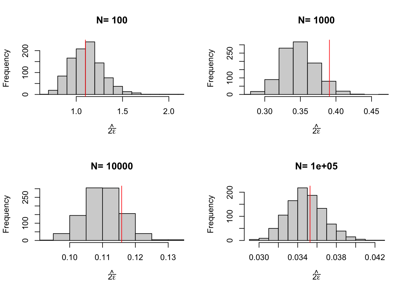
Figure 2.13: Distribution of the bootstrapped approximation of sampling noise over replications of samples of different sizes (true sampling noise in red)
for (k in (1:length(N.sample))){
  table.noise$boot.noise[k] <- mean(simuls.ww.boot[[k]]$boot.samp.noise)
}
ggplot(table.noise, aes(x=as.factor(N), y=TT)) +
  geom_bar(position=position_dodge(), stat="identity", colour='black') +
  geom_errorbar(aes(ymin=TT-sampling.noise/2, ymax=TT+sampling.noise/2), width=.2,position=position_dodge(.9),color='red') +
  geom_errorbar(aes(ymin=TT-boot.noise/2, ymax=TT+boot.noise/2), width=.2,position=position_dodge(.9),color='blue') +
  xlab("Sample Size")+
  theme_bw()
Figure 2.14: Average bootstrapped approximations of sampling noise over replications of samples of different sizes (true sampling noise in red)
N.plot <- 40
plot.list <- list()

for (k in 1:length(N.sample)){
 set.seed(1234)
 test.boot <- simuls.ww.boot[[k]][sample(N.plot),c('WW','boot.lCI','boot.uCI')]
 test.boot <- as.data.frame(cbind(test.boot,rep(samp.noise(simuls.ww.boot[[k]][,'WW'],delta=delta),N.plot)))
 colnames(test.boot) <- c('WW','boot.lCI','boot.uCI','sampling.noise')
 test.boot$id <- 1:N.plot
 plot.test.boot <- ggplot(test.boot, aes(x=as.factor(id), y=WW)) +
     geom_bar(position=position_dodge(), stat="identity", colour='black') +
     geom_errorbar(aes(ymin=WW-sampling.noise/2, ymax=WW+sampling.noise/2), width=.2,position=position_dodge(.9),color='red') +
     geom_errorbar(aes(ymin=boot.lCI, ymax=boot.uCI), width=.2,position=position_dodge(.9),color='blue') +
     geom_hline(aes(yintercept=delta.y.ate(param)), colour="#990000", linetype="dashed")+
     xlab("Sample id")+
     theme_bw()+
     ggtitle(paste("N=",N.sample[k]))
 plot.list[[k]] <- plot.test.boot
}
plot.CI <- plot_grid(plot.list[[1]],plot.list[[2]],plot.list[[3]],plot.list[[4]],ncol=1,nrow=length(N.sample))
print(plot.CI)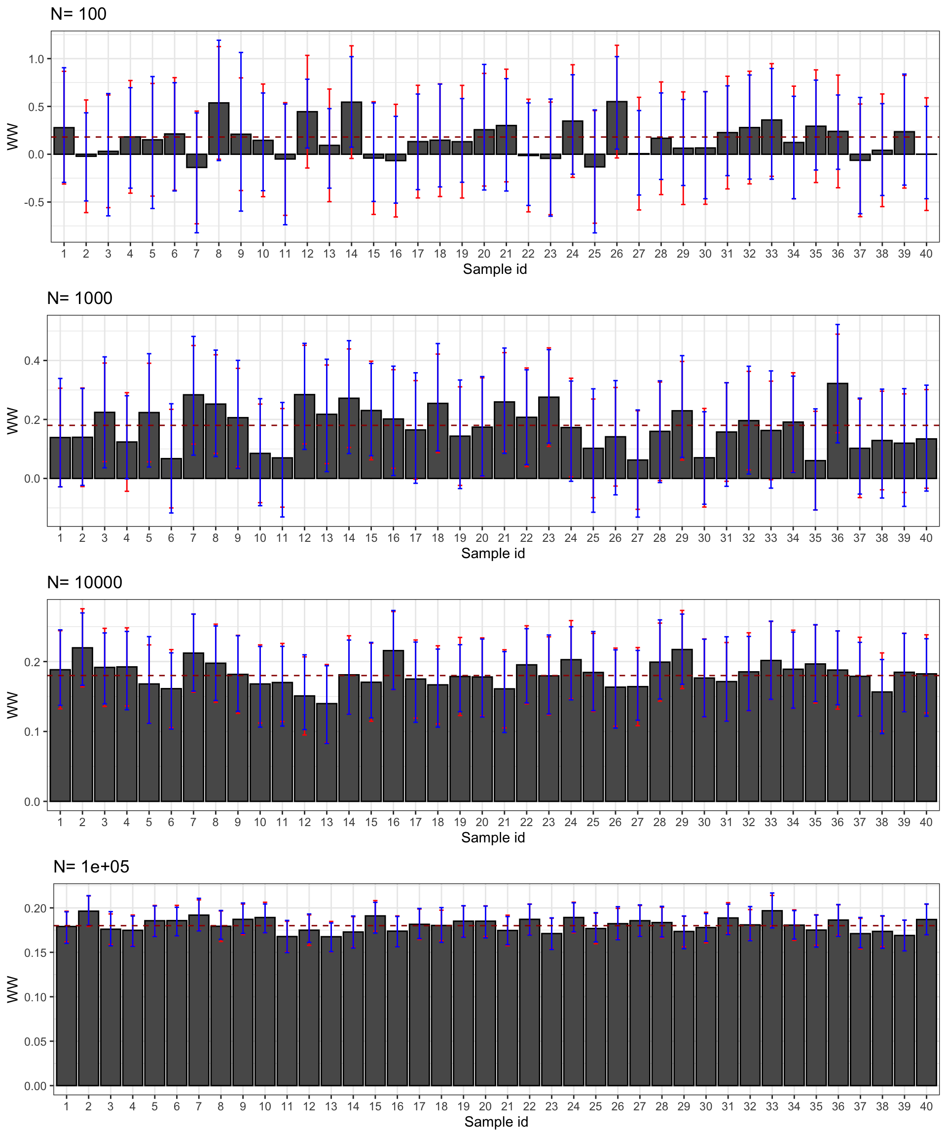
Figure 2.15: Bootstrapped confidence intervals of \(\hat{WW}\) for \(\delta=\) 0.99 over sample replications for various sample sizes (true confidence intervals in red)
TO DO: COMMENT AND USE PIVOTAL TEST STATISTIC
2.2.4.2 Randomization inference
Randomization inference (a.k.a. Fisher’s permutation approach) tries to mimick the sampling noise due to the random allocation of the treatment vector, as we have seen in Section 2.1.3. In practice, the idea is simply to look at how the treatment effect that we estimate varies when we visit all the possible allocations of the treament dummy in the sample. For each new allocation, we are going to compute the with/without estimator using the observed outcomes and the newly allocated treatment dummy. It means that some actually treated observations are going to enter into the computation of the control group mean, while some actually untreated observations are going to enter into the computation of the treatment group mean. As a consequence, the resulting distribution will be centered at zero. Under the assumption of a constant treatment effect, the distribution of the parameter obtained using randomization inference will be an exact estimation of sampling noise for the sample treatment effect.
Notice how beautilful the result is: randomization inference yields an measure of sampling noise. The resulting estimate of sampling noise is not an approximation that is going to become better as sample size increases. No, it is the value of sampling noise in the sample.
There are two ways to compute a confidence interval using Fisher’s permutation approach. One is to form symmetric intervals using our estimate of sampling noise as presented in Section 2.1.4. Another approach is to directly use the quantiles of the distribution of the parameter centered around the estimated treatment effect, in the same spirit as bootstrapped confidence intervals using the percentile approach. This last approach accomodates possible asymetries in the finite sample distribution of the treatment effect.
Computing the value of the treatment effect for all possible treatment allocations can take a lot of time with large samples. That’s why we in general compute the test statistic for a reasonably large number of random allocations.
Remark. Fisher’s original approach is slightly different from the one I delineate here. Fisher wanted to derive a test statistic for whether the treatment effect was zero, not to estimate sampling noise. Under the null that the treatment has absolutely no effect whatsoever on any unit, any test statistic whose value should be zero if the two distributions where identical can be computed on the actual sample and its distribution can be derived using Fisher’s permutation approach. The test statistic can be the difference in means, standard deviations, medians, ranks, the T-stat, the Kolmogorov-Smirnov test statistic or any other test statistic that you might want to compute. Comparing the actual value of the test statistic to its distribution under the null gives a p-value for the validity of the null.
Remark. Imbens and Rubin propose a more complex procedure to derive the confidence interval for the treatment effect using randomization inference. They propose to compute Fisher’s p-value for different values of the treatment effect, and to set the confidence interval as the values of the treatment effect under and above which the p-value is smaller than \(\delta\). When using the with/without estimator as the test statistic, the two approches should be equivalent. Is is possible that the estimates using statistics less influenced by outliers are more precise though.
Remark. Note that we pay two prices for having an exact estimation of sampling noise:
- We have to assume that the treatment effect is constant, e.g. we have to assume homoskedasticity. This is in general not the case. Whether this is in general a big issue depends on how large the difference is between homoskedastic and heteroskedastic standard errors. One way around this issue would be to add a small amount of noise to the observations that are in the group with the lowest variance. Whether this would work in practice is still to be demonstrated.
- We have to be interested only in the sampling noise of the sample treatment effect. The sampling noise of the population treatment effect is not estimated using Fisher’s permutation approach. As we have seen in Section 2.1.3, there is no practical difference between these two sampling noises in our example. Whether this is the case in general deserves further investigation.
Example 2.10 In practice, randomization inference is very close to a bootstrap procedure, except that instead of resampling with replacement from the original sample, we only change the vector of treatment allocation at each replication.
fisher.fun.ww.1 <- function(seed,data){
  set.seed(seed,kind="Wichmann-Hill")
  data$D <- rbinom(nrow(data),1,mean(data$Ds))
  ols.ww <- lm(y~D,data=data)
  ww <- ols.ww$coef[[2]]
  return(ww)
}

fisher.fun.ww <- function(Nfisher,data,delta){
  fisher <- unlist(lapply(1:Nfisher,fisher.fun.ww.1,data=data))
  ols.ww <- lm(y~Ds,data=data)
  ww <- ols.ww$coef[[2]]
  fisher <- fisher+ ww
  fisher.CI.ww <- c(quantile(fisher,prob=(1-delta)/2),quantile(fisher,prob=(1+delta)/2))
  fisher.samp.noise.ww <- quantile(fisher,prob=(1+delta)/2)-quantile(fisher,prob=(1-delta)/2)
  return(list(fisher,fisher.CI.ww,fisher.samp.noise.ww))
}

Nfisher <- 500
ww.fisher <- fisher.fun.ww(Nfisher,data,delta)
Over 500 replications, the 99% confidence interval based on Fisher’s permutation approach is \(\left\{-0.052;0.3\right\}\). As a consequence, the bootstrapped estimate of 99% sampling noise is of 0.352. Remember that, with \(N=\) 1000, sampling noise is actually equal to 0.39.
In order to assess the global precision of Fisher’s permutation method, we are going to resort to Monte Carlo simulations.
monte.carlo.ww.fisher <- function(s,N,param,Nfisher,delta){
  set.seed(s)
  mu <- rnorm(N,param["barmu"],sqrt(param["sigma2mu"]))
  UB <- rnorm(N,0,sqrt(param["sigma2U"]))
  yB <- mu + UB
  YB <- exp(yB)
  Ds <- rep(0,N)
  V <- rnorm(N,param["barmu"],sqrt(param["sigma2mu"]+param["sigma2U"]))
  Ds[V<=log(param["barY"])] <- 1
  epsilon <- rnorm(N,0,sqrt(param["sigma2epsilon"]))
  eta<- rnorm(N,0,sqrt(param["sigma2eta"]))
  U0 <- param["rho"]*UB + epsilon
  y0 <- mu +  U0 + param["delta"]
  alpha <- param["baralpha"]+  param["theta"]*mu + eta
  y1 <- y0+alpha
  Y0 <- exp(y0)
  Y1 <- exp(y1)
  y <- y1*Ds+y0*(1-Ds)
  Y <- Y1*Ds+Y0*(1-Ds)
  data <- as.data.frame(cbind(y,Ds,yB))
  ww.fisher <- fisher.fun.ww(Nfisher,data,delta)
  return(c((1/sum(Ds))*sum(y*Ds)-(1/sum(1-Ds))*sum(y*(1-Ds)),var(y[Ds==1]),var(y[Ds==0]),mean(Ds),ww.fisher[[2]][1],ww.fisher[[2]][2],ww.fisher[[3]]))
}

sf.simuls.ww.N.fisher <- function(N,Nsim,Nfisher,delta,param){
  sfInit(parallel=TRUE,cpus=2*ncpus)
  sfExport("fisher.fun.ww","fisher.fun.ww.1")
  sim <- as.data.frame(matrix(unlist(sfLapply(1:Nsim,monte.carlo.ww.fisher,N=N,Nfisher=Nfisher,delta=delta,param=param)),nrow=Nsim,ncol=7,byrow=TRUE))
  sfStop()
  colnames(sim) <- c('WW','V1','V0','p','fisher.lCI','fisher.uCI','fisher.samp.noise')
  return(sim)
}

simuls.ww.fisher <- lapply(N.sample,sf.simuls.ww.N.fisher,Nsim=Nsim,param=param,Nfisher=Nfisher,delta=delta)
We can now graph our bootstrapped estimate of sampling noise in all of our samples, the average bootstrapped estimates of sampling noise and of confidence intervals, as Figures 2.16, 2.17 and 2.18 show. The results are pretty good. On average, estimates of sampling noise using Randomization Inference are pretty accurate, as Figure 2.17 shows. It seems that sampling noise is underestimated by Randomization Inference when \(N=\) 1000, without any clear reason why.
par(mfrow=c(2,2))
for (i in 1:4){
  hist(simuls.ww.fisher[[i]][,'fisher.samp.noise'],main=paste('N=',as.character(N.sample[i])),xlab=expression(hat(2*bar(epsilon))),xlim=c(min(simuls.ww.fisher[[i]][,'fisher.samp.noise']),max(simuls.ww.fisher[[i]][,'fisher.samp.noise'])))
  abline(v=table.noise[i,colnames(table.noise)=='sampling.noise'],col="red")
}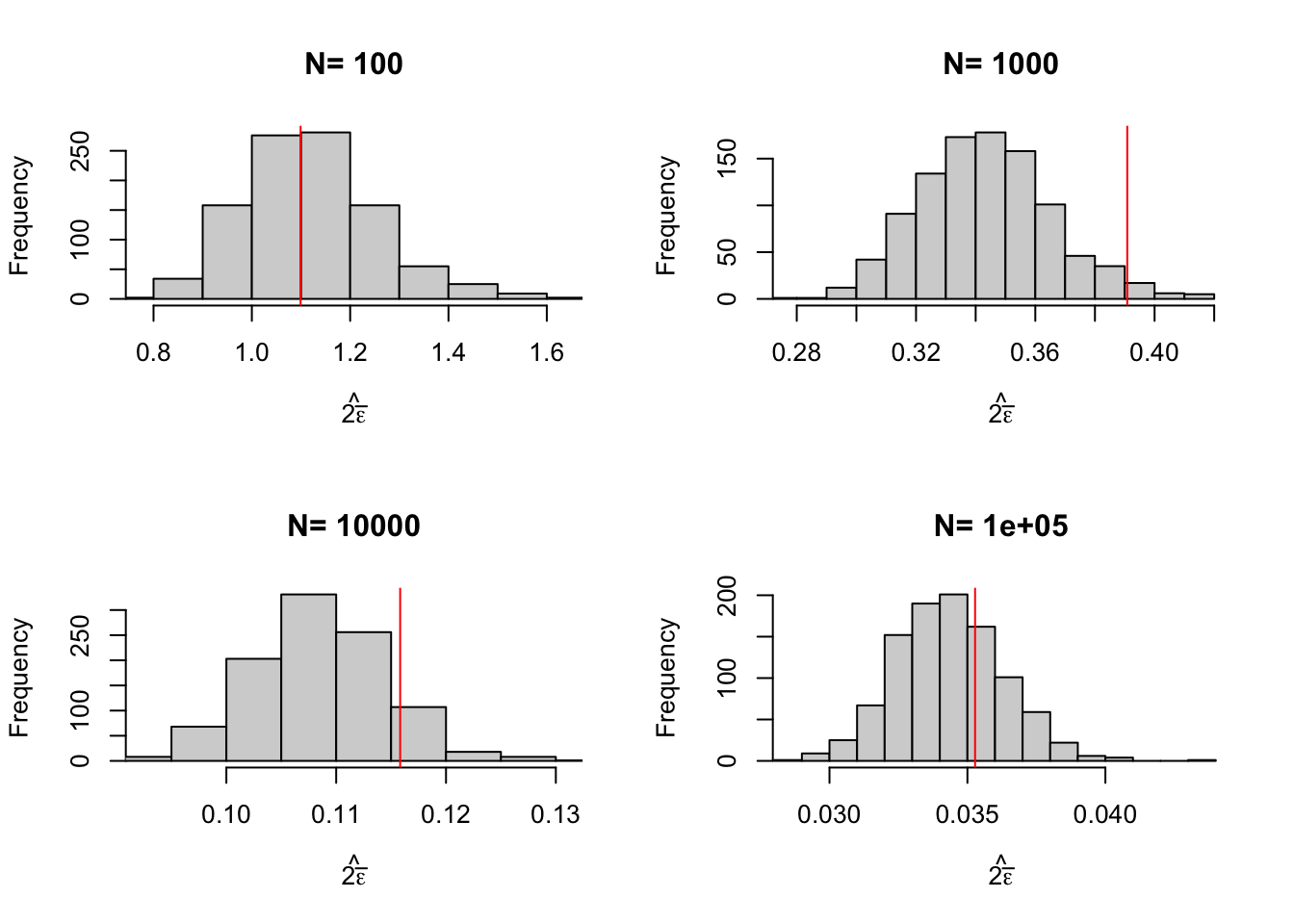
Figure 2.16: Distribution of the estimates of sampling noise using Randomization Inference over replications of samples of different sizes (true sampling noise in red)
for (k in (1:length(N.sample))){
  table.noise$fisher.noise[k] <- mean(simuls.ww.fisher[[k]]$fisher.samp.noise)
}
ggplot(table.noise, aes(x=as.factor(N), y=TT)) +
  geom_bar(position=position_dodge(), stat="identity", colour='black') +
  geom_errorbar(aes(ymin=TT-sampling.noise/2, ymax=TT+sampling.noise/2), width=.2,position=position_dodge(.9),color='red') +
  geom_errorbar(aes(ymin=TT-fisher.noise/2, ymax=TT+fisher.noise/2), width=.2,position=position_dodge(.9),color='blue') +
  xlab("Sample Size")+
  theme_bw()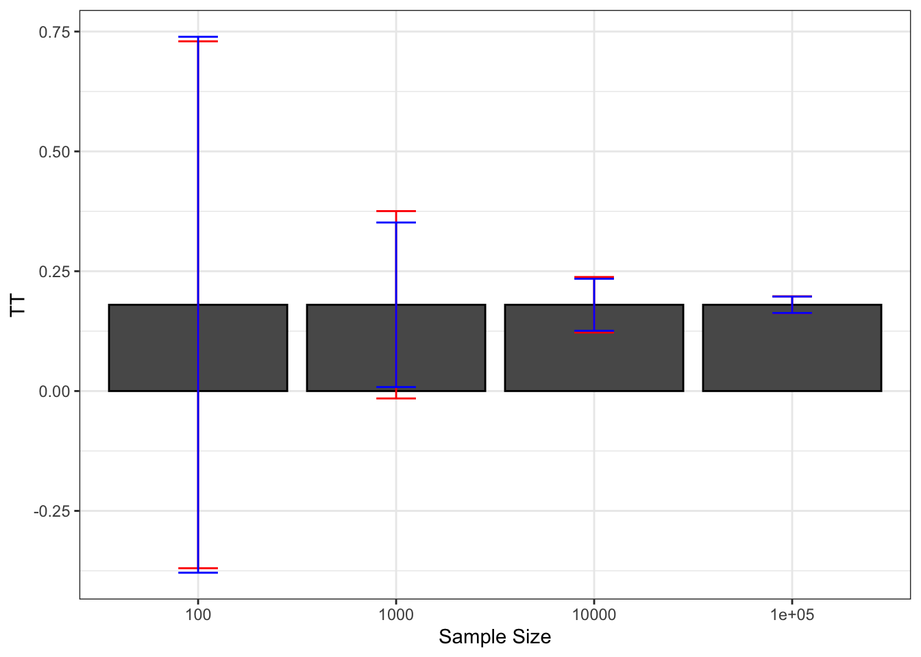
Figure 2.17: Average estimates of sampling noise using Randomization Inference over replications of samples of different sizes (true sampling noise in red)
N.plot <- 40
plot.list <- list()

for (k in 1:length(N.sample)){
 set.seed(1234)
 test.fisher <- simuls.ww.fisher[[k]][sample(N.plot),c('WW','fisher.lCI','fisher.uCI')]
 test.fisher <- as.data.frame(cbind(test.fisher,rep(samp.noise(simuls.ww.fisher[[k]][,'WW'],delta=delta),N.plot)))
 colnames(test.fisher) <- c('WW','fisher.lCI','fisher.uCI','sampling.noise')
 test.fisher$id <- 1:N.plot
 plot.test.fisher <- ggplot(test.fisher, aes(x=as.factor(id), y=WW)) +
     geom_bar(position=position_dodge(), stat="identity", colour='black') +
     geom_errorbar(aes(ymin=WW-sampling.noise/2, ymax=WW+sampling.noise/2), width=.2,position=position_dodge(.9),color='red') +
     geom_errorbar(aes(ymin=fisher.lCI, ymax=fisher.uCI), width=.2,position=position_dodge(.9),color='blue') +
     geom_hline(aes(yintercept=delta.y.ate(param)), colour="#990000", linetype="dashed")+
     xlab("Sample id")+
     theme_bw()+
     ggtitle(paste("N=",N.sample[k]))
 plot.list[[k]] <- plot.test.fisher
}
plot.CI <- plot_grid(plot.list[[1]],plot.list[[2]],plot.list[[3]],plot.list[[4]],ncol=1,nrow=length(N.sample))
print(plot.CI)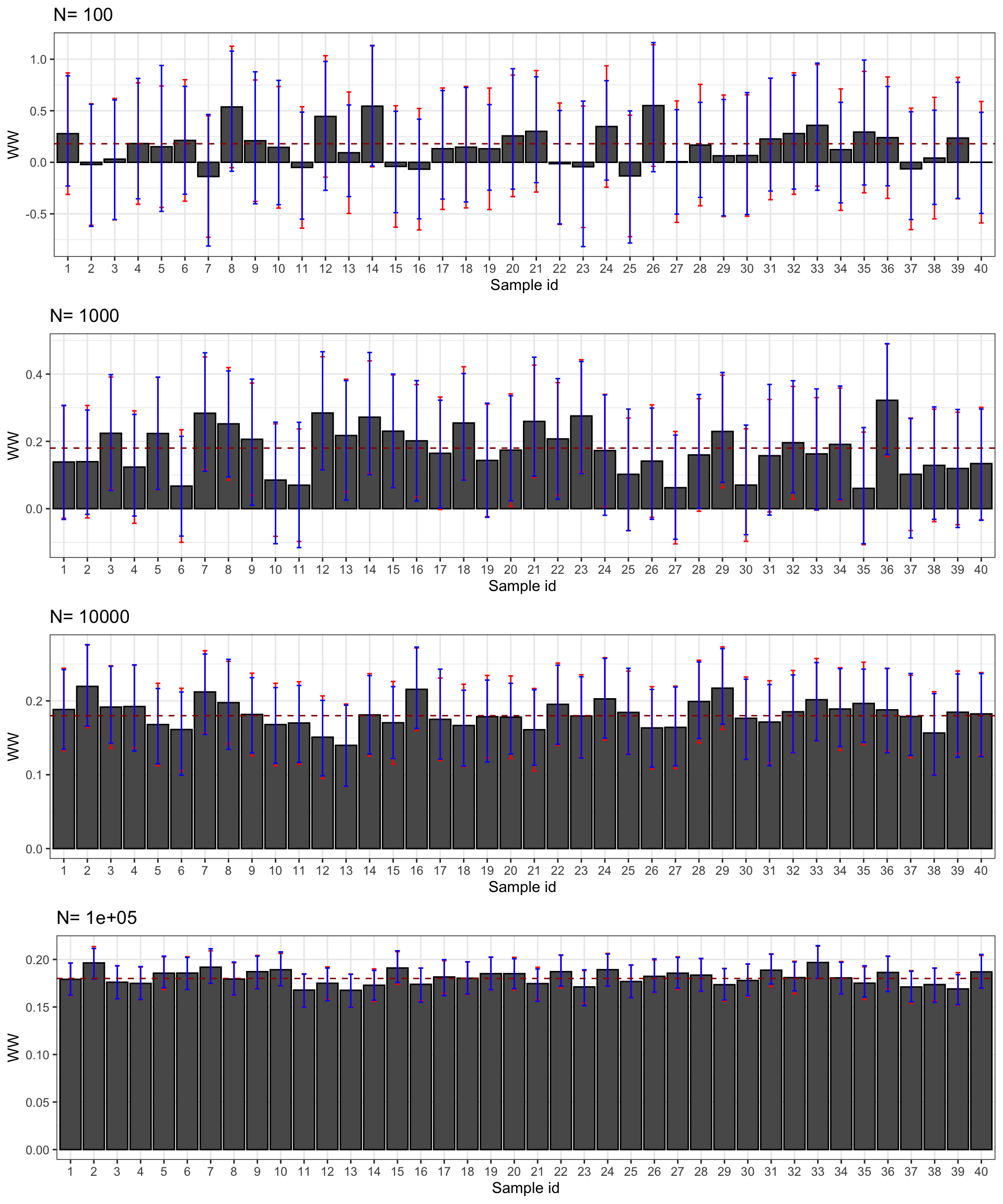
Figure 2.18: Confidence intervals of \(\hat{WW}\) for \(\delta=\) 0.99 estimated using Randomization Inference over sample replications for various sample sizes (true confidence intervals in red)
TO DO: ALTERNATIVE APPROACH USING p-VALUES