Chapter 9 Clustering
Until now, we have assumed throughout the book that different units, say \(i\) and \(j\), with \(i\neq j\), never interact in any way. One way we have encoded that is by implicitly assuming that the treatment of individual \(i\) has no impact on the outcomes of individual \(j\). We will clarify this assumption in Chapter 11, and study ways to relax it. Another way we have assumed an absence of interactions is by assuming that all potential outcomes and treatment indicators are independently and identically distributed across observations. We have encoded this restriction at various points, first with Assumption 2.2 in the context of estimating the sampling noise in Randomized Controlled Trials, and then with Assumptions 4.15 and 4.17 in DID settings. This assumption enabled us to leverage the Central Limit Theorem, the most powerful tool we can use to derive asymptotic approximations to our estimators.
The i.i.d. assumption is nevertheless extremely restrictive. It excludes various cases that we are likely to encouter in real life scenarios. For example, this assumption will be wrong if we allocate the treatment at the level of a group of units, such as a village or a firm for example. Groups of units are generally called clusters. In that case, the treatment indicator will not be i.i.d. across observations, since knowing the treatment status of a unit in a given cluster can help us predict the treatment status of its neighbors in the same cluster, so Assumption 2.2 would be violated. The i.i.d. assumption will also be wrong in panel data with repeated observations of the same units if the outcomes are correlated over time for reasons other than having a fixed effect in common. For example, any case in which shocks to outcomes around the fixed effect are somewhat persistent over time, we will have correlation between the observations of the same unit over time, and between the changes in outcomes of the same unit over time. This last issue would violate Assumption 4.15. There are many instances where the shocks to outcomes are likely correlated over time, such as productivity shocks, earnings, education, health, savings, etc, that is most of the outcomes we are generally interested in. Finally, the i.i.d. assumption will also be violated in DID settings in repeated cross sections if the treatment is allocated at a more aggregate level than that of the individual unit. For example, if we study the consequences of laws that vary at the levels of U.S. counties or States, such as minimum wage laws for example, and we have observations on firm’s TFP and employment level, or on individuals’ earnings, then we have correlations between the treatment status of units belonging to the same cluster, and probably the outcomes are correlated as well between the units in the same cluster.
In this chapter, we are going to examine what happens to our traditional estimators when relaxing the i.i.d. assumption, and which new estimators we can use, and what types of diagnostic tests we can make use of in order to assess the severity of the issue. Clustering, as this issue is generally called, has been the topic of a very large literature in econometrics, whose results are sometimes vague, sometimes hard to comprehend or to reconcile, etc. What we are going to do is to try to carve a path through this literature, trying to enlighten its main motivations, its main tools and its main results. We are first going to study the case of clustering in the context of Randomized Controlled Trials. We will then move on to the case of temporal autocorrelation in panel data and we will end with the case of panel data with clustering across time and between observations in each cross section.
9.1 Clustering in Randomized Controlled Trials
What I propose is to first start to see what the problem of clustering does to sampling noise, and how much our default estimator of sampling noise assuming no clustering is biased. I will then introduce the notion of design effect, which is a way to quantify the effect of clustering on sampling noise estimates. Finally, I will propose ways to provide estimates of sampling noise that account for clustering.
9.1.1 An example
Let us first see how that happens in our example before deriving the reason for why we have such a problem and the possible solutions. For that, we are going to simulate data with clusters (such as villages) and we are going to have two features of he data generating process that happen at the cluster level:
- The treatment is going to be randomized at the cluster level. We thus have a clustered randomized controlled trial, where randomization is at the level of clusters regrouping several individual units of observation. For example, think of a classroom where we randomize a new treatment and we observe outcomes at the student level (grades, health status, participation, etc), or think of a cvaccination camoaign randomized at the village level.
- The outcome is going to be autocorrelated within clusters. For example, think of the common determinants of school success (such as the teacher, the parents, the overall conditions at the school) or of the health status in a village (climate, sanitation, pressure by parasites, etc) at the cluster level. These common determinants make the outcomes of two people taken at random in a given cluster more similar than those of two people taken at random in the whole population. The share of the variance in outcomes explained by the variance across clusters is called the intra-cluster correlation coefficient (ICC) and is going to play a key role in what follows.
Example 9.1 Let’s see how we model all of that in our example. We choose to generate the outcomes of individual \(i\) in cluster \(c\) in period \(t\) as follows:
\[\begin{align*} y^0_{i,c,t} & = \mu_{i,c} + U_{i,t} \\ \mu_{i,c} & = \mu^C_c + \mu^U_i \\ U_{i,t} & = \rho U_{i,t-1} + \epsilon_{i,t}, \end{align*}\]
where \(U_{i,0}\), \(\epsilon_{i,t}\), \(\mu^U_i\) and \(\mu_c\) are i.i.d. shocks independent of each other. I introduce a panel data structure because it will be useful for the simulations in the next section.
\(\mu_c\) is the error term varying at the cluster level. We call it a cluster fixed effect. The intra-cluster correlation coefficient is equal to the ratio between the variance in outcomes between clusters and the total variance in outcomes:
\[\begin{align*} ICC_t & = \frac{\sigma^2_{\mu_c}}{\sigma^2_{\mu^c}+\sigma^2_{\mu^U}+\sigma^2_{U_t}}. \end{align*}\]
Let’s generate some data and see what an increase in ICC does to our estimates of the treatment effect in a Brute Force design. As usual, we are going to use the With/Without estimator to compute the treatment effect. Let us first set parameter values:
param <- c(8,.5,.28,1500,0.9,0.01,0.05,0.05,0.05,0.1)
names(param) <- c("barmu","sigma2mu","sigma2U","barY","rho","theta","sigma2epsilon","sigma2eta","delta","baralpha")
Let us then simulate one dataset:
N <- 1000
ICC.mu <- 0.2
Nclusters <- 100

set.seed(1234)
# I am going to draw a cluster fixed effect
muC <- rnorm(Nclusters,0,sqrt(param["sigma2mu"]*ICC.mu))
muC <- rep(muC,each=N/Nclusters)
# I draw an individual fixed effect with the remaining variance
muU <- rnorm(N,0,sqrt(param["sigma2mu"]*(1-ICC.mu)))
mu <- param["barmu"] + muC + muU
UBB <- rnorm(N,0,sqrt(param["sigma2U"]))
yBB <- mu + UBB
YBB <- exp(yBB)
epsilonB <- rnorm(N,0,sqrt(param["sigma2epsilon"]))
U0B <- param["rho"]*UBB + epsilonB
y0B <- mu +  U0B
epsilonA <- rnorm(N,0,sqrt(param["sigma2epsilon"]))
U0A <- param["rho"]*U0B + epsilonA
y0A <- mu +  U0A + param["delta"]
eta<- rnorm(N,0,sqrt(param["sigma2eta"]))
alpha <- param["baralpha"]+  param["theta"]*mu + eta
y1B <- y0B+alpha
y1A <- y0A+alpha

# randomized allocation at the cluster level
Rs <- runif(Nclusters)
# cluster level treatment vector
Rc <- ifelse(Rs<=.5,1,0)
# individual level treatment vector
R <- rep(Rc,each=N/Nclusters)

# outcomes
yB <- y0B
yA <- y1A*R+y0A*(1-R)

# clusters
cluster <- 1:Nclusters
cluster <- rep(cluster,each=N/Nclusters)
Let us finally run a set of Monte Carlo simulations, varying ICC:
monte.carlo.BF.ICC <- function(s,N,Nclusters,ICC.mu,param){
  set.seed(s)
  # I am going to draw a cluster fixed effect
  muC <- rnorm(Nclusters,0,sqrt(param["sigma2mu"]*ICC.mu))
  muC <- rep(muC,each=N/Nclusters)
  # I draw an individual fixed effect with the remaining variance
  muU <- rnorm(N,0,sqrt(param["sigma2mu"]*(1-ICC.mu)))
  mu <- param["barmu"] + muC + muU
  UBB <- rnorm(N,0,sqrt(param["sigma2U"]))
  yBB <- mu + UBB
  YBB <- exp(yBB)
  epsilonB <- rnorm(N,0,sqrt(param["sigma2epsilon"]))
  U0B <- param["rho"]*UBB + epsilonB
  y0B <- mu +  U0B
  epsilonA <- rnorm(N,0,sqrt(param["sigma2epsilon"]))
  U0A <- param["rho"]*U0B + epsilonA
  y0A <- mu +  U0A + param["delta"]
  eta<- rnorm(N,0,sqrt(param["sigma2eta"]))
  alpha <- param["baralpha"]+  param["theta"]*mu + eta
  y1B <- y0B+alpha
  y1A <- y0A+alpha

  # randomized allocation at the cluster level
  Rs <- runif(Nclusters)
  # cluster level treatment vector
  Rc <- ifelse(Rs<=.5,1,0)
  # individual level treatment vector
  R <- rep(Rc,each=N/Nclusters)

  # outcomes
  yB <- y0B
  yA <- y1A*R+y0A*(1-R)

  # regression
  ols.ww.BF <- lm(yA ~ R)
  ols.ww.BF.yB <- lm(yA ~ R + yB)

  # True ICC
  data <- as.data.frame(cbind(yB,R))
  cluster <- 1:Nclusters
  cluster <- rep(cluster,each=N/Nclusters)
  data$cluster <- cluster
  data <- group_by(data,cluster)
  data <- merge(data,summarise(data,yB.mean=mean(yB)))
  ICC <- var(data$yB.mean)/var(yB)

  return(c(ols.ww.BF$coef[[2]],ols.ww.BF.yB$coef[[2]],ICC))
}

sf.simuls.BF.ICC <- function(ICC.mu,N,Nclusters,Nsim,param){
  sfInit(parallel=TRUE,cpus=8)
  sfLibrary(dplyr)
  sim <- matrix(unlist(sfLapply(1:Nsim,monte.carlo.BF.ICC,N=N,Nclusters=Nclusters,ICC.mu=ICC.mu,param=param)),nrow=Nsim,ncol=3,byrow=TRUE)
  sfStop()
  colnames(sim) <- c('BF','BF.yB','ICC')
  return(sim)
}

Nsim <- 1000
#Nsim <- 50
ICC.val <- c(0,0.05,0.2,0.5,0.8,1)

simuls.BF.ICC <- lapply(ICC.val,sf.simuls.BF.ICC,N=N,Nclusters=Nclusters,Nsim=Nsim,param=param)
names(simuls.BF.ICC) <- ICC.val
Let us now present the results of the simulations:
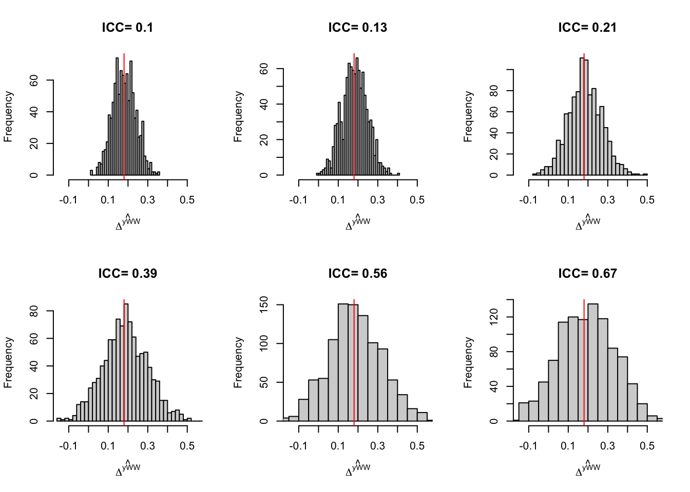
Figure 9.1: Distribution of the \(WW\) estimator in a Brute Force Design for various levels of ICC
Figure 9.1 suggests that increasing the ICC increases sampling noise. Let’s compute sampling noise formally:
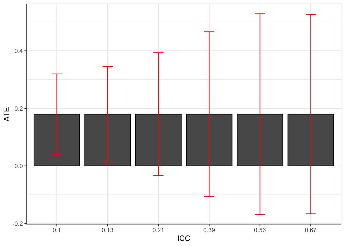
Figure 9.2: Effect of ICC on the 99% sampling noise of the WW estimator in a Brute Force design
Figure 9.2 confirms that increasing the ICC increases sampling noise in a major way. With a small ICC, sampling noise is equal to 0.28, while it is equal to 0.69 with the largest ICC. The difference is more than sizable.
Increasing the ICC is equivalent to losing sample size. The intuition for this result is that, with autocorrelated data, the Central Limit Theorem applies at a much slower pace. The part of the error term that is common to all observations in a given cluster only vanishes as we add more clusters, not as we add more observations per cluster. As a result, this part of sampling noise decreases with the square root of the number of clusters, not with the square root of the number of observations.
The second result to emerge from Figure 9.2 is that ignoring clustering would severely underestimate sampling noise. The lower level of sampling noise on Figure 9.2 is roughly equal to the level of sampling noise that an estimator ignoring clustering would deliver (the estimator detailed in Theorem 2.5). Let’s compute the naive estimator of sampling noise based on Theorem 2.5:
The naive estimate of sampling noise is thus 0.3.
9.1.2 Design effect
A very useful way to understand what clustering does to sampling noise is to derive the variance of the With/Without estimator in the presence of clustering of a simple nature: when all the outcomes within a cluster are correlated in the same way and correlation between outcomes is zero outside of the clusters and all clusters have the same size. This derivation enables us to introduce the notion of design effect, which is a way to quantify the effect of clustering on sampling noise estimates as a function of the ICC. In order to make this derivation, we need to formally specify the covariance matrix of our error terms.
Let us assume that we have access to observations about \(N\) units, allocated in \(n\) clusters of equal size \(m\). Among the \(n\) clusters, \(n_1\) are treated and \(n_0\) are in the control group. Let \(R_{i}\) denote the randomized allocation variable for each unit \(i\), which takes value one when unit \(i\) is located in a cluster \(c\) that has been (randomly) allocated to the treatment and value zero otherwise. Let \(R^C_{c}\) denote the randomized allocation variable for each cluster \(c\), which takes value one when cluster \(c\) has been (randomly) allocated to the treatment and value zero otherwise. Let \(\mathbf{R}_c\) be the vector of randomized allocations at the cluster level: it has length equal to \(n\), and each value is equal to \(R^C_{c}\). Let us denote \(U_i^1=Y_i^1-\esp{Y_i^1|R_{i}=1}\) and \(U_i^0=Y_i^0-\esp{Y_i^0|R_{i}=0}\) and \(U_i=R_{i}U_i^1+(1-R_{i})U_i^0\). Let \(U\) be the vector of all \(U_i\) error terms. Let \(\sigma^2_1=\var{U_i^1}\) and \(\sigma^2_0=\var{U_i^0}\). Finally, let \(\Omega_1\) and \(\Omega_0\) be \(m\times m\) matrices with a diagonal of one and off-diagonal terms all equal to \(\rho_1\) and \(\rho_0\) respectively, with \(\rho_1\) and \(\rho_0\) the Intra-Cluster Correlation Coefficient among the treated and untreated observation respectively. We are now equipped to relax Assumption 2.2:
Hypothesis 9.1 (Clustered Design) We assume that the error terms are clustered:
\[\begin{align*} \esp{UU'} & = \sigma^2_1\diag{\mathbf{R}_c}\otimes\Omega_1+\sigma^2_0(I-\diag{\mathbf{R}_c})\otimes\Omega_0. \end{align*}\]
Remark. Assumption 9.1 imposes that the covariance structure between potential outcomes is block diagonal. That is that there is the same correlation between outcomes for observations in the same cluster, and there is no correlation between outcomes for observations that do not belong to the same cluster.
Theorem 9.1 (Variance of the With/Without estimator under Clustering) Under Assumptions 1.7, 2.1 and 9.1,
\[\begin{align*} \var{{\hat{\Delta^Y_{WW}}}} & = \frac{1}{N}\left(\frac{\sigma^2_0}{1-\Pr(R_i=1)}(1+(m-1)\rho_0)+\frac{\sigma^2_1}{\Pr(R_i=1)}(1+(m-1)\rho_1)\right). \end{align*}\]
Proof. See in Appendix A.5.1.
We can also prove the following corollary:
Corollary 9.1 (Design Effect) Under Assumptions 1.7, 2.1 and 9.1, and with \(\rho_0=\rho_1=\rho\), we have:
\[\begin{align*} \var{{\hat{\Delta^Y_{WW}}}} & = \frac{1}{N}(1+(m-1)\rho)\left(\frac{\sigma^2_0}{1-\Pr(D_i=1)}+\frac{\sigma^2_1}{\Pr(D_i=1)}\right), \end{align*}\]
with \((1+(m-1)\rho)\) the design effect.
Proof. The proof is straightforward using Theorem 9.1.
Remark. Note that the formula for the variance of the \(WW\) estimator in Corollary 9.1 is equal to the formula for the variance of the same estimator under Assumption 2.2 of i.i.d. error terms derived in Lemma A.5 multiplied by the design effect. As soon as \(m>1\), the design effect is strictly superior to one, meaning that the variance of the \(WW\) estimator in a clustered design is superior to the variance of the \(WW\) estimator in a designed where randomization is done at the unit level. The larger the Intra Cluster Correlation Coefficient \(\rho\) and the higehr the number of units per cluster \(m\), the larger the design effect.
Remark. One very useful way to think about the design effect is to think about effective sample size \(N^*=\frac{N}{1+(m-1)\rho}\) as being the sample size that would yield the same precision as our clustered experiment but with an experiment randomized at the unit level. In that sense, the design effect measures by how much clustering decreases our effective sample size.
Example 9.2 It is possible to visualize the extent of the design effect is to plot the effective sample size as a function of the real sample size, for various values of \(\rho\) and \(m\). For that, we simply need to generate a function to compute the effective sample size.
DesignEffect <- function(rho,m){
  return(1+(m-1)*rho)
}
EffSampleSize <- function(N,...){
  return(N/DesignEffect(...))
}
Let us now plot the result:
ggplot()+
  xlim(0,10000) +
  ylim(0,10000) +
  geom_function(aes(linetype="m=2 and rho=0.1",color="m=2 and rho=0.1"),fun=EffSampleSize,args=list(rho=0.1,m=2)) +
  geom_function(aes(linetype="m=5 and rho=0.1",color="m=5 and rho=0.1"),fun=EffSampleSize,args=list(rho=0.1,m=5)) +
  geom_function(aes(linetype="m=10 and rho=0.1",color="m=10 and rho=0.1"),fun=EffSampleSize,args=list(rho=0.1,m=10)) +
  geom_function(aes(linetype="m=2 and rho=0.5",color="m=2 and rho=0.5"),fun=EffSampleSize,args=list(rho=0.5,m=2)) +
  geom_function(aes(linetype="m=5 and rho=0.5",color="m=5 and rho=0.5"),fun=EffSampleSize,args=list(rho=0.5,m=5)) +
  geom_function(aes(linetype="m=10 and rho=0.5",color="m=10 and rho=0.5"),fun=EffSampleSize,args=list(rho=0.5,m=10)) +
  geom_function(aes(linetype="m=2 and rho=1",color="m=2 and rho=1"),fun=EffSampleSize,args=list(rho=1,m=2)) +
  geom_function(aes(linetype="m=5 and rho=1",color="m=5 and rho=1"),fun=EffSampleSize,args=list(rho=1,m=5)) +
  geom_function(aes(linetype="m=10 and rho=1",color="m=10 and rho=1"),fun=EffSampleSize,args=list(rho=1,m=10)) +
  geom_abline(slope=1,intercept=0,linetype="dotted",color='black')+
  scale_color_discrete(name="") +
  scale_linetype_discrete(name="") +
  ylab("Effective sample size") +
  xlab("Actual sample size") +
  theme_bw()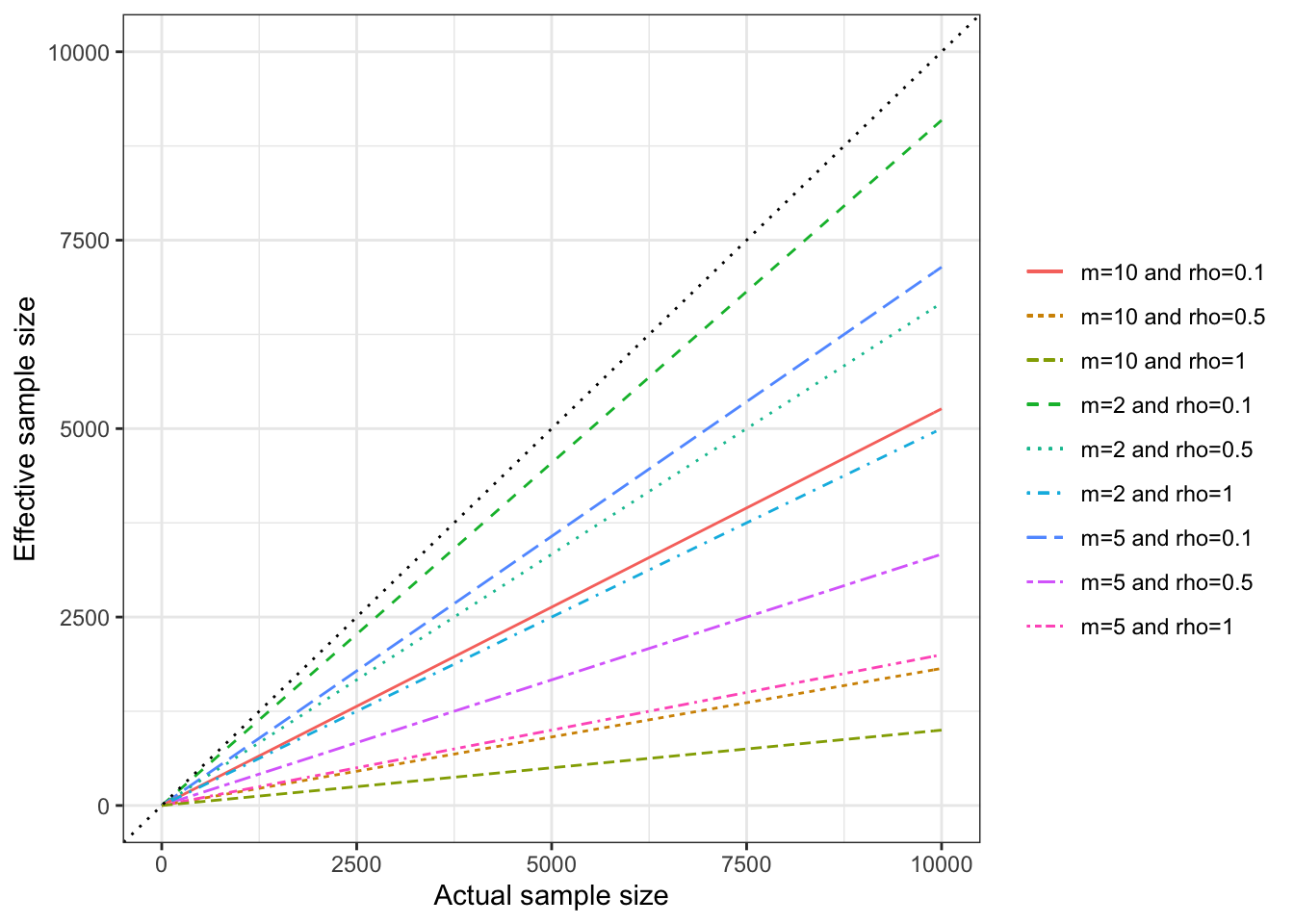
Figure 9.3: Effective sample size in a clustered design
Figure 9.3 shows that effective sample size can decrease enormously because of clustering. For example, with clusters of size \(m=10\), and the Intra Cluster Correlation Coefficient \(\rho=0.5\), a sample size of \(N=10000\) observations is equivalent to an unclustered RCT ran on a sample of \(N^*=\) 1818, which is equivalent to dividing the true sample size by 5.5.
Discuss clustering in the power analysis chapter
9.1.3 Estimating sampling noise accounting for clustering
We have shown that clustering increases sampling noise around our estimates and worse, that our basic estimates of sampling noise based on the i.i.d. assumption underestimate the true amount of sampling noise, sometimes severely. Devising ways to estimate sampling noise that offer a correct estimate of the true extent of sampling noise in the presence of clustering is thus a very important endeavor, if we are to gauge correctly the precision of our treatment effect estimates. Let us see several ways to do that.
Remark. There exists several super cool resources which detail the topics of estimating standard errors under clustering. I really like the one by Cameron and Miller (2015). The one by McKinnon, Nielsen and Webb (2023) is also nice, even if more technical.
9.1.3.1 Using the plug-in formula
One direct and simple way to account for clustering is to use the formula in Theorem 9.1 or the simpler formula in Corollary 9.1. The Intra Cluster Correlation Coefficient can be computed as the ratio of the variance of the mean of the outcomes at the cluster level divided by the total variance of the outcomes in the sample. Once we have an estimate of the variance of the treatment effect, we can build sampling noise \(2\epsilon\) by multiplying the resulting standard error by \(2\Phi^{-1}\left(\frac{\delta+1}{2}\right)\).
Remark. Note that this approach implicitly assumes that the Central Limit Theorem holds with clustered data. Actually, in the clustered case, as long as we allow the number of clusters to go to infinity, we can safely use the classical CLT. We will also see in Section 9.7 that versions of the CLT exist for more general case where there is dependency between data points.
Remark. One uncertainty with the approach relying on CLT based on increasing the number of clusters is that we are unsure whether the normalizing constant in the CLT is \(N\), the total sample size, or \(n\), the number of clusters. This will be rigorously clarified in Sections 9.8 and 9.7.
Example 9.3 In practice, to apply the formula in Theorem 9.1, we simply need to compute the total variance of outcomes in the treated and control groups, and to estimate the Intra Cluster Correlation Coefficients of outcomes among the treated and the controls respectively, \(\rho_1\) and \(\rho_0\). The Intra Cluster Correlation Coefficient can be computed as the ratio of the variance of the mean of the outcomes at the cluster level divided by the total variance of the outcomes in the sample. Let’s go.
# Function for the plug in variance estimator
VarClusterPlugIn <- function(sigma1,sigma0,ICC1,ICC0,p,m,N){
  dEffect0 <- 1+(m-1)*ICC0
  dEffect1 <- 1+(m-1)*ICC1
  return((dEffect0*sigma0/(1-p)+dEffect1*sigma1/p)/N)
}

# Preparing data
dataCluster <- data.frame(Cluster=cluster,yA=yA,yB=yB,R=R)
# Computing ICC
# Cluster-level variance
VaryAClus <- dataCluster %>%
                group_by(R,Cluster) %>%
                summarize(
                  MeanyAClus = mean(yA)
                ) %>%
                ungroup(.) %>%
                group_by(R) %>%
                summarize(
                  VaryAClus = var(MeanyAClus)
                )
# Total variance
VaryA <- dataCluster %>%
          group_by(R) %>%
          summarize(
            VaryATot = var(yA)
          )
# ICC
ICC <- VaryA %>%
        left_join(VaryAClus,by='R') %>%
        mutate(
          ICC =  VaryAClus/VaryATot
        )
# p
p <- mean(dataCluster$R)
# Variance estimate
VarClusteredWW <- VarClusterPlugIn(sigma1=ICC %>% filter(R==1) %>% pull(VaryATot),
                                   sigma0=ICC %>% filter(R==0) %>% pull(VaryATot),
                                   ICC1=ICC %>% filter(R==1) %>% pull(ICC),
                                   ICC0=ICC %>% filter(R==0) %>% pull(ICC),
                                   p=p,
                                   m=N/Nclusters,
                                   N=N)
Our estimate of sampling noise accounting for clustering using the plug-in estimator is equal to 0.53. The true level of sampling noise estimated from the simulations is 0.43. Remember that the naive estimate of sampling noise which ignores clustering is 0.3.
9.1.3.2 Using cluster-robust standard errors
The most widely used approach for accounting for clustering when estimating treatment effects is using cluster-robust standard errors. We start with the formula for the variance of the OLS estimator, that we have derived in the proof of Theorem 9.1: \(\var{\hat{\Theta}_{OLS}|X}=(X'X)^{-1}X'\esp{UU'|X}X(X'X)^{-1}\). The basic idea of clustered robust standard errors is to build an empirical estimate of the covariance matrix of the residuals \(\esp{UU'|X}\) using the estimated residuals \(\hat{U}_i\). We might want to use the full \(\mathbf{\hat{U}}\mathbf{\hat{U}}'\) matrix, with \(\mathbf{\hat{U}}\) the vector of all estimated residuals, but that would not work, because, by construction, the OLS estimator produces residuals which are orthogonal to the covariates, so that \(X'\esp{UU'|X}X\) is a null matrix.
Instead, cluster-robust standard errors are estimated by assuming first that the matrix \(\esp{UU'|X}\) is block diagonal, meaning that observations are only correlated within clusters. Let \(\mathbf{\hat{U}}_c\) be the vector of empirical residuals of observations residing in cluster \(c\). Let’s write \(\hat{\Omega}_c=\mathbf{\hat{U}}_c\mathbf{\hat{U}}_c'\) and \(\hat{\Omega}=\diag(\left\{\hat{\Omega}_c\right\}_{c=1}^n)\). We can now use \(\hatvar{\hat{\Theta}_{OLS,Clustered}}=(X'X)^{-1}X'\hat{\Omega}X(X'X)^{-1}\) as our cluster-robust estimate of the covariance matrix of the OLS estimator, with \(\Theta=(\alpha,\beta)\) the parameter vector in the equation \(Y_i=\alpha+\beta R_i+U_i\), where \(\beta=\Delta^Y_{WW}\), as Lemma A.3 shows.
In practice, some authors and statistical software might add a degrees of freedom correction to these estimates as a way to curb small sample bias. One common correction factor is \(\frac{n}{n-1}\frac{N-1}{N-k}\) with \(K\) the number of covariates. Another classical correction is \(\frac{n}{n-1}\).
Example 9.4 Let’s see how these approaches work in our example.
The most straightforward way to implement the cluster-robust variance estimator in R is to use the vcovCL command from the sandwich package.
The type option of vcovCL can take values HC0, where the only correction is \(\frac{n}{n-1}\), and HC1, where the correction is \(\frac{n}{n-1}\frac{N-1}{N-k}\).
Another approach is to use the feols function of the fixest package with the cluster option.
# regression
RegBFCLuster <- lm(yA ~ R, data=dataCluster)
# cluster-robust standard error
VCovClusterHC1 <- vcovCL(RegBFCLuster,cluster=~cluster,type="HC1",sandwich=TRUE)
VCovClusterHC0 <- vcovCL(RegBFCLuster,cluster=~cluster,type="HC0",sandwich=TRUE)
# using fixest
RegBFCLusterFixest <- feols(yA ~ R | 1, data=dataCluster, cluster="Cluster")
With the HC1 correction, our estimate of sampling noise accounting for clustering using the plug-in estimator is equal to 0.46, and to 0.46 with the HC0 correction and to 0.46 with fixest.
The true level of sampling noise estimated from the simulations is 0.43.
Remember that the naive estimate of sampling noise which ignores clustering is 0.3.
9.1.3.3 Using Feasible Generalized Least Squares
As Cameron and Miller (2015) remark, when error terms are autocorrelated, the OLS estimator is not the most efficient one, and a Generalized Least Squares (GLS) estimator could perform better. The problem is to find the Feasible Generalized Least Squares estimator that makes real this potential gain in precision. In order to derive it, we have first to specify a model for \(\Omega_{GLS}=\esp{UU'|X}\). One such model is the one in Assumption 9.1. Under such a model, we know that the GLS estimator of the parameter vector \(\Theta=(\alpha,\beta)\) in the equation \(Y_i=\alpha+\beta R_i+U_i\) is \(\hat{\Theta}_{GLS}=(X'\Omega_{GLS}^{-1}X)^{-1}X'\Omega_{GLS}^{-1}Y\). With a consistent estimator for \(\Omega\), e.g. \(\hat{\Omega}_{FGLS}\), we have \(\hat{\Theta}_{FGLS}=(X'\hat{\Omega}_{FGLS}^{-1}X)^{-1}X'\hat{\Omega}_{FGLS}^{-1}Y\) with the associated estimated variance: \(\hatvar{\hat{\Theta}_{FGLS}}=(X'\hat{\Omega}_{FGLS}^{-1}X)^{-1}\). Cameron and Miller (2015) also suggest that we can build a cluster robust estimate of the variance of the FGLS estimator as follows: \(\hatvar{\hat{\Theta}_{FGLS,Clustered}}=(X'\hat{\Omega}_{FGLS}^{-1}X)^{-1}X'\hat{\Omega}_{FGLS}^{-1}\hat{\Omega}\hat{\Omega}_{FGLS}^{-1}X(X'\hat{\Omega}_{FGLS}^{-1}X)^{-1}\), with \(\hat{\Omega}=\diag(\left\{\hat{\Omega}_c\right\}_{c=1}^n)\), \(\hat{\Omega}_c=\mathbf{\hat{U}}_c\mathbf{\hat{U}}_c'\) and \(\mathbf{\hat{U}}_c\) be the vector of empirical residuals of observations residing in cluster \(c\), as in the previous section, but obtained with the FGLS model now.
Remark. As Cameron and Miller (2015) remark, the approach of building a cluster-robust estimator for the variance of the FGLS estimator has been popularized in biostatistics by Liang and Zeger (1986).
Example 9.5 Let’s see how the FGLS approach works in our example. Following Assumption 9.1, we know that \(\hat{\Omega}_{FGLS}=\hat{\sigma}^2_1\diag{\mathbf{R}_c}\otimes\hat{\Omega}_1+\hat{\sigma}^2_0(I-\diag{\mathbf{R}_c})\otimes\hat{\Omega}_0\), with \(\hat{\sigma}^2_1\) the estimated variance of outcomes in the treated group, \(\hat{\sigma}^2_0\), the estimated varianc of outcomes in the control group and \(\hat{\Omega}_1\) and \(\hat{\Omega}_0\) matrices with a diagonal of one and off-diagonal elements equal to \(\hat{\rho}_1\) and \(\hat{\rho}_0\), respectively, the Intra Cluster Correlation Coefficient of outcomes in the treated and untreated groups respectively. We know how to estimate all these parameters so we can build \(\hat{\Omega}_{FGLS}\). Let’s do it.
# Omega matrix at the cluster level
Omega1 <- matrix(data=ICC %>% filter(R==1) %>% pull(ICC),nrow=N/Nclusters,ncol=N/Nclusters) + diag(1-ICC %>% filter(R==1) %>% pull(ICC),nrow=N/Nclusters,ncol=N/Nclusters)
Omega0 <- matrix(data=ICC %>% filter(R==0) %>% pull(ICC),nrow=N/Nclusters,ncol=N/Nclusters) + diag(1-ICC %>% filter(R==0) %>% pull(ICC),nrow=N/Nclusters,ncol=N/Nclusters)
# sigma1 and sigma0
sigma21 <- ICC %>% filter(R==1) %>% pull(VaryATot)
sigma20 <- ICC %>% filter(R==0) %>% pull(VaryATot)
# OmegaFGLS matrix at teh sample level
OmegaFGLS <- sigma21*diag(Rc)%x%Omega1 +sigma20*(diag(1,nrow=Nclusters,ncol=Nclusters)-diag(Rc))%x%Omega0
# Inverting Omega
InvOmegaFGLS <- solve(OmegaFGLS)
# matrix of covariates
X <- cbind(1,R)
# FGLS estimator
RegFGLS <- solve((t(X)%*%InvOmegaFGLS%*%X))%*%(t(X)%*%InvOmegaFGLS%*%yA)
# FGLS estimate of WW
WWyFGLS <- RegFGLS[2,1]
# Basic variance estimate of the FGLS estimator
VcovRegFGLS <- solve((t(X)%*%InvOmegaFGLS%*%X))
# estimated basic standard error of WWyFGLS
SeWWyFGLS <- sqrt(VcovRegFGLS[2,2])
The FGLS estimator of the treatment effect is equal to 0.24 \(\pm\) 0.2 with \(\delta=0.95\). This means that the basic FGLS estimate of sampling noise is equal to 0.53. The true level of sampling noise estimated from the simulations is 0.43.
Let us now try to estimate the cluster robust variance of the FGLS estimator.
This requires to compute the matrix \(\hat{\Omega}_c=\mathbf{\hat{U}}_c\mathbf{\hat{U}}_c'\) for each cluster.
For that, we are going to extract the block diagonal matrix \(\hat{\Omega}=\mathbf{\hat{U}}\mathbf{\hat{U}}'\) using the package diagonal.
# computing FGLS residuals
ResidFGLS <- yA-X%*%RegFGLS
# Product of residuals matrix
HatOmega <- ResidFGLS%*%t(ResidFGLS)
# block diagonal equal to zero
diagonals::fatdiag(HatOmega,size=N/Nclusters) <- 0
# take the UU' matrix and take of the OFF diagonal elements
HatOmega <- ResidFGLS%*%t(ResidFGLS)-HatOmega

# compute the Cluster robust FGLS variance matrix estimator
VcovRegFGLSCluster <- VcovRegFGLS%*%t(X)%*%InvOmegaFGLS%*%HatOmega%*%InvOmegaFGLS%*%X%*%VcovRegFGLS
# estimated clustered standard error of WWyFGLS
SeWWyFGLSCluster <- sqrt(VcovRegFGLSCluster[2,2])
This means that the cluster-robust FGLS estimate of sampling noise is equal to 0.46. The true level of sampling noise estimated from the simulations is 0.43.
9.1.3.4 Using the Bootstrap
The bootstrap is a data-intensive non-parametric way to obtain cluster-robust estimates of sampling noise. Here, we are going to use the non-parametric bootstrap, but other bootstrap methods exist. Cameron and Miller (2015) cover some of them.
Remark. A key distinction when we use the bootstrap is whether it can offer asymptotic refinements or not.
The way we implement the non-parametric (or pair) bootstrap is as follows:
- We build a sample of \(N_c\) clusters by sampling with replacement from the original sample,
- For each sample \(b\), we estimate a treatment effect \(\hat{\Delta}^y_{WW}(b)\),
- After computing \(B\) such estimates, we compute the bootstrap-cluster-robust variance estimator as follows:
\[\begin{align*} \hatvar{\hat{\Delta}^y_{WW}}^{Bootstrap}_{Clustered} & = \frac{1}{B-1}\sum_{b=1}^B\left(\hat{\Delta}^y_{WW}(b)-\frac{1}{B}\sum_{b=1}^B\hat{\Delta}^y_{WW}(b)\right)^2. \end{align*}\]
Example 9.6 Let’s see how this works in our example. We first need to generate a dataset with outcomes, treatment and cluster indicators. Then we need to draw repeatedly new vectors of clusters identifiers, with replacement, and compute the WW estimator for each.
# Regroup data and cluster id
# already done in dataCluster
# write a function to draw a new vector of clusters and return the WW estimator
# seed: the seed for the PRNG
# data: the dataset
# cluster: the name of the cluster variable (with cluster variable indexed from 1 to Nc)
# y: the name of the outcome variable
# D: the name of the treatment variable
NPBootCluster <- function(seed,data,cluster,y,D){
  # set seed
  set.seed(seed)
  # compute number of clusters
  NClusters <- data %>%
                group_by(!!sym(cluster)) %>%
                summarize(count=n()) %>%
                summarize(NClusters=n())
  # draw a sample with replacement
  SampleClusters <- data.frame(BootClusters =sample(1:(NClusters[[1]]),size=NClusters[[1]],replace=TRUE)) %>%
                      left_join(data,by=c('BootClusters'=cluster))
  # run regression
  RegCluster <- lm(as.formula(paste(y,D,sep='~')),data=SampleClusters)
  # WW estimate
  WW <- coef(RegCluster)[[2]]
  # return
  return(WW)
}

# testing
test <- NPBootCluster(seed=1,data=dataCluster,cluster='Cluster',y='yA',D='R')
# programming to run in parallel
sf.NP.Boot.Cluster <- function(Nsim,...){
  sfInit(parallel=TRUE,cpus=8)
  sfLibrary(dplyr)
  sim <- matrix(unlist(sfLapply(1:Nsim,NPBootCluster,data=dataCluster,cluster='Cluster',y='yA',D='R')),nrow=Nsim,ncol=1,byrow=TRUE)
  sfStop()
  colnames(sim) <- c('WW')
  return(sim)
}
# Number of simulations
#Nsim <- 10
Nsim <- 400
# running in parallel
simuls.NP.Boot.Cluster <- sf.NP.Boot.Cluster(Nsim=Nsim,data=dataCluster,cluster='Cluster',y='yA',D='R')
## R Version: R version 4.1.1 (2021-08-10)
##
## Library dplyr loaded.The cluster-robust non-parametric bootstrap estimate of sampling noise is equal to 0.48. The true level of sampling noise estimated from the simulations is 0.43.
9.1.3.5 Using Randomization inference
Randomization inference is a different way to obtain estimates of the true level of sampling noise using resampling estimates. One intuitive way of running randomization inference would be to draw new vectors of treatment status at the cluster level and estimate the variability of treatment effect estimates. One problem with that approach is that it does not take into account the fact that treated and control differ by the amount of the treatment effect and that is going to add some additional noise in the estimate. A more rigorous approach follows the suggestion in Imbens and Rubin (2015), Section 5.7 and proceed as follows:
- Assume a size for the treatment effect (let’s call it \(\tau\))
- Compute each potential outcome for each treated (\(\tilde{Y}_i^0=Y_i-\tau\) and \(\tilde{Y}_i^1=Y_i\)) and each untreated (\(\tilde{Y}_i^1=Y_i+\tau\) and \(\tilde{Y}_i^0=Y_i\)) unit in the original sample
- Draw a new treatment allocation \(\tilde{R}^1_i\)
- Compute the realized outcomes \(\tilde{Y}_i=\tilde{Y}_i^1\tilde{R}^1_i+\tilde{Y}_i^0(1-\tilde{R}^1_i)\)
- Compute the \(WW\) estimate \(\tilde{\Delta}^Y_{WW_1}\) using the new treatment allocation \(\tilde{R}^1_i\) and the realized outcomes \(\tilde{Y}_i\)
- Repeat the operation \(\tilde{N}\) times, to obtain \(\left\{\tilde{\Delta}^Y_{WW_k}\right\}_{k=1}^{\tilde{N}}\)
- Compute the empirical p-value \(\tilde{p}(\tau)\) as the proportion of sample draws where \(\left|\tilde{\Delta}^Y_{WW_k}-\tau\right|\leq\left|\hat{\Delta}^Y_{WW}-\tau\right|\), where \(\hat{\Delta}^Y_{WW}\) is the treatment effect estimate in the original sample.
- Repeat for various values of \(\tau\) on a set of points \(\tau_1,\dots,\tau_{K}\).
- Find the values \(\tau^u_{\alpha}\) and \(\tau^l_{\alpha}\) that are such that \(\tilde{p}(\tau^u_{\alpha})\approx\alpha\approx\tilde{p}(\tau^l_{\alpha})\) and \(\tau^l_{\alpha}<\hat{\Delta}^Y_{WW}<\tau^u_{\alpha}\). \(\left[\tau^l_{\alpha},\tau^u_{\alpha}\right]\) is the \(1-\alpha\) cluster robust randomizaiton inference-based confidence interval for \(\hat{\Delta}^Y_{WW}\).
Example 9.7 Let’s see how that works in our example.
# function computing one randomization inference draw for one value of tau
# s: the seed for the PRNG
# data: the dataset
# cluster: the name of the cluster variable (with cluster variable indexed from 1 to Nc)
# y: the name of the outcome variable
# D: the name of the treatment variable
ClusteredRI <- function(s,tau,data,cluster,y,D){
  # Compute potential outcomes
  data <- data %>%
            mutate(
              y0 = case_when(
                !!sym(D)==1 ~ !!sym(y)-tau,
                !!sym(D)==0 ~ !!sym(y),
                TRUE ~ 99
              ),
              y1 = case_when(
                !!sym(D)==1 ~ !!sym(y),
                !!sym(D)==0 ~ !!sym(y)+tau,
                TRUE ~ 99
              )
            )
  # drawing alternative treatment vector at cluster level
  # compute number of clusters
  NClusters <- data %>%
                group_by(!!sym(cluster)) %>%
                summarize(count=n()) %>%
                ungroup(.) %>%
                summarize(NClusters=n())
  # set seed
  set.seed(s)
  # randomized allocation at the cluster level
  Rs <- runif(NClusters[[1]])
  # cluster level treatment vector
  Rc <- ifelse(Rs<=.5,1,0)
  # dataframe of treated joined to original data
  RIdata <- data.frame(ClusterId=1:NClusters[[1]],Rc=Rc) %>%
            left_join(data,by=c("ClusterId"=cluster)) %>%
            #generating RI observed outcomes
            mutate(
              yc = y0*(1-Rc)+y1*Rc
            )
  # estimating the RI WW treatment effect
  RegWWRI <- lm(yc~Rc,data=RIdata)
  # returning estimate
  return(coef(RegWWRI)[[2]])
}

# testing
testRI <- ClusteredRI(s=1,tau=0,data=dataCluster,cluster='Cluster',y='yA',D='R')
# testing sapply
Nsim <- 10
testRIapply <- sapply(1:Nsim,ClusteredRI,tau=0,data=dataCluster,cluster='Cluster',y='yA',D='R')

# parallelize for one value of tau
# programming to run in parallel
sf.RI.Cluster <- function(Nsim,tau,data,cluster,y,D){
  sfInit(parallel=TRUE,cpus=8)
  sfLibrary(dplyr)
  sfExport('dataCluster')
  sim <- matrix(unlist(sfLapply(1:Nsim,ClusteredRI,tau=tau,data=data,cluster=cluster,y=y,D=D)),nrow=Nsim,ncol=1,byrow=TRUE)
  sfStop()
  colnames(sim) <- c('WW')
  return(sim)
}
# testing
sf.test.RI <- sf.RI.Cluster(Nsim=Nsim,tau=0,data=dataCluster,cluster='Cluster',y='yA',D='R')

# lapply over values of tau on a grid
# function that takes tau as an input and spits out the empirical p-value
# tau: hypothesized value of treatment effect
# WWhat: estimated vamlue of treatment effect in the original sample
ParallelClusteredRI <- function(tau,WWhat,...){
  # computing the RI distribution of WW estimates for given tau
  sf.WW.RI <- sf.RI.Cluster(tau=tau,...)
  # estimate enpirical cdf of |WWRI-tau|
  F.WW.RI.tau <- ecdf(abs(sf.WW.RI-tau))
  # Compute the p-value
  pvalue <- 1-F.WW.RI.tau(abs(WWhat-tau))
  # return the p-value
  return(pvalue)
}
# testing
testRItau <- ParallelClusteredRI(tau=0,WWhat=0.2,Nsim=Nsim,data=dataCluster,cluster='Cluster',y='yA',D='R')
# run on a grid of tau's
tau.grid <- seq(from=-0.15,to=0.55,by=0.01)
Nsim <- 1000
simuls.RI.tau <- sapply(tau.grid,ParallelClusteredRI,WWhat=0.2,Nsim=Nsim,data=dataCluster,cluster='Cluster',y='yA',D='R')
names(simuls.RI.tau) <- tau.grid
# putting results in data frame
RI.pvalues.tau <- data.frame(pvalue=simuls.RI.tau,tau=tau.grid)
Let us visualize the resulting estimates of the p-values as a function of \(\tau\):
ggplot(RI.pvalues.tau,aes(x=tau,y=pvalue))+
  geom_point() +
  geom_line() +
  geom_hline(yintercept = 0.05,linetype='dotted',color='red')+
  ylim(0,1) +
  ylab("p-value") +
  xlab(expression(tau)) +
  theme_bw()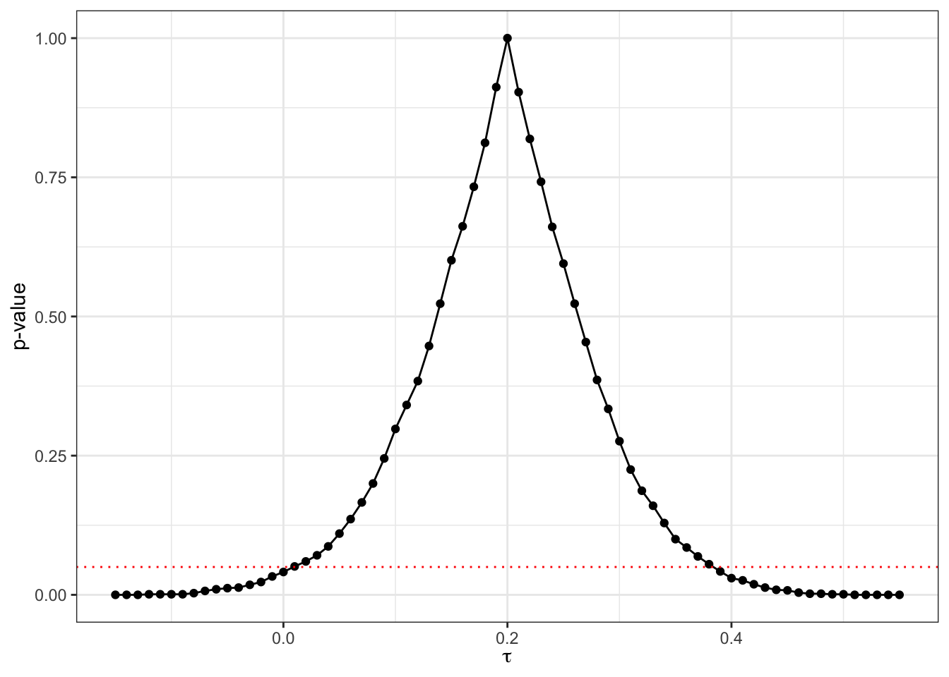
Figure 9.4: Randomization inference p-values as a function of \(\tau\)
Let us now compute the confidence interval and estimate of sampling noise:
# computing RI-based confidence interval and sampling noise estimate
# function that takes a dataframe of pvalues and a grid and spits out both ends of confidence interval and level delta and sampling noise
# delta: level of the confidence interval (95% or 99% for example)
# data: a data frame with a variable for tau and a variable for pvalues
# tau: name of the tau variable
# pval: name of the pvalue variable
RI.CI <- function(delta,data,tau,pval){
  data <- data %>%
            mutate(
              # finding observations with pvalue lower than delta
              below.pval = case_when(
                !!sym(pval) <= 1-delta ~ 1,
                !!sym(pval) > 1-delta ~ 0,
                TRUE ~99
              ),
              # finding observations below the tau with maximum pvalue
              max.pval = max(!!sym(pval)),
              max.pval.tau = case_when(
                !!sym(pval) == max.pval ~ !!sym(tau),
                TRUE ~ -Inf
              ),
              max.pval.tau = max(max.pval.tau),
              below.max.paval.tau = case_when(
                tau<max.pval.tau ~ 1,
                tau>=max.pval.tau ~ 0,
                TRUE ~ Inf
              )
            ) %>%
            # keeping only observations that are below pval of delta%
            filter(below.pval==1) %>%
            # grouping by whether tau is above or below the tau with maximum pvalue
            group_by(below.max.paval.tau)
  # finding max and min values that are extremes of delta% CI
  minCI <- data %>%
            filter(below.max.paval.tau==1) %>%
            ungroup(.) %>%
            summarize(
              minCI = max(!!sym(tau))
            ) %>%
            pull(minCI)
  maxCI <- data %>%
            filter(below.max.paval.tau==0) %>%
            ungroup(.) %>%
            summarize(
              maxCI = min(!!sym(tau))
            ) %>%
            pull(maxCI)
  # results
  results <- list(minCI,maxCI,maxCI-minCI)
  names(results) <- c("LowCI","HighCI","SamplingNoise")
  return(results)
}
# test
testRICI95 <- RI.CI(delta=0.95,data=RI.pvalues.tau,tau='tau',pval='pvalue')
testRICI99 <- RI.CI(delta=0.99,data=RI.pvalues.tau,tau='tau',pval='pvalue')
As a result of our procedure, the randomization inference based 95% confidence interval for the \(WW\) estimator is \(\left[\right.\) 0 , 0.39 \(\left.\right]\) and the 99% sampling noise is equal to 0.5.
The true level of sampling noise estimated from the simulations is 0.43.
Remark. Another, simpler, option for implementing randomization inference would have been simply to reallocate the treatment vector among clusters and keep the original values of the outcomes instead of generating the outcomes under the null for each value of \(\tau\). This is the simple approach we have used in Chapter 2. The properties of this approach have not been studied to my knowledge, but it would be interest!ing to know under which conditions it is approximately correct. Let’s check what would have happened if we had used this simpler approach to randomization inference.
# function computing one simplified randomization inference draw
# s: the seed for the PRNG
# data: the dataset
# cluster: the name of the cluster variable (with cluster variable indexed from 1 to Nc)
# y: the name of the outcome variable
# D: the name of the treatment variable
ClusteredRISimple <- function(s,data,cluster,y){
  # drawing alternative treatment vector at cluster level
  # compute number of clusters
  NClusters <- data %>%
                group_by(!!sym(cluster)) %>%
                summarize(count=n()) %>%
                ungroup(.) %>%
                summarize(NClusters=n())
  # set seed
  set.seed(s)
  # randomized allocation at the cluster level
  Rs <- runif(NClusters[[1]])
  # cluster level treatment vector
  Rc <- ifelse(Rs<=.5,1,0)
  # dataframe of treated joined to original data
  RIdata <- data.frame(ClusterId=1:NClusters[[1]],Rc=Rc) %>%
            left_join(data,by=c("ClusterId"=cluster))
  # estimating the RI WW treatment effect
  RegWWRISimple <- lm(as.formula(paste(y,'Rc',sep='~')),data=RIdata)
  # returning estimate
  return(coef(RegWWRISimple)[[2]])
}

# testing
testRISimple <- ClusteredRISimple(s=1,data=dataCluster,cluster='Cluster',y='yA')
# testing sapply
Nsim <- 10
testRISimpleapply <- sapply(1:Nsim,ClusteredRISimple,data=dataCluster,cluster='Cluster',y='yA')

# programming to run in parallel
sf.RI.Cluster.Simple <- function(Nsim,data,cluster,y){
  sfInit(parallel=TRUE,cpus=8)
  sfLibrary(dplyr)
  sim <- matrix(unlist(sfLapply(1:Nsim,ClusteredRISimple,data=data,cluster=cluster,y=y)),nrow=Nsim,ncol=1,byrow=TRUE)
  sfStop()
  colnames(sim) <- c('WW')
  return(sim)
}
# testing
sf.test.RI.simple <- sf.RI.Cluster.Simple(Nsim=Nsim,data=dataCluster,cluster='Cluster',y='yA')
# running
Nsim <- 1000
simuls.RI.Simple <- sf.RI.Cluster.Simple(Nsim=Nsim,data=dataCluster,cluster='Cluster',y='yA')
Var.WW.RI.Simple <- var(simuls.RI.Simple)
With the simplified randomization inference procedure, the 99% sampling noise is equal to 0.49.
The true level of sampling noise estimated from the simulations is 0.43.
9.2 Clustering in panel data
Another source of clustering appears in panel data, where we follow the same observation over time. One way to account for the correlation between the outcomes of the same individual over time is to add individual level fixed effects, and to use either a within estimator or a Least Squares Dummy Variable estimator, as we did in Section 4.3. But adding individual level fixed effects probably does not account for the overall correlation between observations of the same individual over time. A case in point is autocorrelation in the error terms due to persistent shocks. If a unit has experienced a shock at date \(t\), she is more likely to experience a similar shock at date \(t+1\). For example, health problems do not solve themselves miraculously between survey rounds. In the same manner, job loss or job changes or hurricanes, etc, all have effects that persist over time. As a consequence, we often believe that the observations for the same unit are correlated over time, abve and beyond what can be captured by a unit fixed effect. In this section, we are going to study the issue of clustering in panel data, focusing on the estimators we have studied in Section 4.3, especially the simple DID estimator, the fixed effects estimator, and the Sun and Abraham estimator in staggered designs. A key result of importance is that DID estimates which only involve two-periods are not affected by the autocorrelation problem, while estimates which aggregate more than two periods of data are affected, and the more so as they aggregate more time periods. We are first going to take an example to exemplify the importance of the problem. We will then derive the closed form variance of the various estimators under simplified assumptions on the autocorrelation between error terms. Finally, we will explain how to estimate sampling noise in panel data with autocorrelated error terms.
9.2.1 An example
Let us start with an example of how autocorrelated error terms alter the precision of panel data estimates. For that, we are going to generate long time series of panel data and explore how the variability of treatment effect estimates changes with persistence in error terms at the individual level, both for the event-study estimates (which rely on \(2\times 2\) comparisons) and for the TT estimate, which relies on aggregated treatment effects. For simplicity, we are going to jave a design without staggered entry, but everything we are saying here applies to staggered entry as well.
Check what happens with staggered entry
I am going to use the following model:
We model outcomes dynamics as follows:
\[\begin{align*} Y_{i,t} & = D_{i,t}Y^1_{i,t}+(1-D_{i,t})Y_{i,t}^0\\ Y_{i,t}^1 & = Y_{i,t}^0 + \bar\alpha \\ Y_{i,t}^0 & = \mu_i + U_{i,t} \\ U_{i,t} & = \rho U_{i,t-1} +\epsilon_{i,t} \\ D_{i,t} & = \uns{D^*_{i,k}\geq0}\uns{t\geq k} \\ D^*_{i,k} & = \theta_i + \eta_{i,k}. \end{align*}\]
Outcome dynamics are characterized by an individual fixed effect \(\mu_i\) and an AR(1) process with autoregressive parameter \(\rho\in\left[0,1\right]\). \(\epsilon_{i,t}\) is i.i.d. and has finite variance \(\sigma^2\) and is independent from all the other variables in the model. \(U_{i,0}\) has finite variance \(\sigma^2_{U_0}\) and is independent from all the other variables in the model. The program is only available at period \(k\). Participation in the program (which we denote \(D_{i,t}\)) depends on the utility from entering the program \(D^*_{i,k}\) being positive. \(\eta_{i,k}\) is a random shock uncorrelated with any of the other variables in the model. Selection bias occurs because \(\mu_i\) and \(\theta_i\) are correlated.
Let us now choose some parameter values (but the value of \(\rho\)):
# basic parameter values
param.basic <- c(0.05,0.72,0.55,0.55,0.5,0.1,0)
names(param.basic) <- c("sigma","sigmaU0","sigmamu","sigmatheta","rhosigmamutheta","sigmaeta","baralpha")
Note that I have chosen the true effect of the treatment to be zero, which saves me computational difficulties because \(Y_{i,t}=Y^0_{i,t}\), and does not matter at all for now since we are trying to estimate sampling noise and not the treatment effect itself. Let us now encode a function generating one sample for one choice of parameter values and seed and spitting out one estimate of the event study parameters and of the TT parameter based on Sun and Abraham estimator. I am going also to estimate the \(2\times 2\) DID estimator along with its heteroskedasticity robust standard errors, both as a within estimator and as a first-difference estimator, in order to check whether the standard error estimates are similar in all three approaches.
# function generating a sample of outcomes for K time periods with N sample size and spitting out DID estimates (both event study and TT, with both Sunab and )
# seed: seed setting the PRNG
# N: number of units in the panel
# K: number of periods in the panel
# k: treatment date
# param: basic parameters
# rho: value of rho
# cluster: whether we cluster or not our treatment effect estimates for temporal autocorrelation ("None", vs "Temporal")
Outcome.Sample.DID.Long <- function(seed,N,K,k,param,rho,cluster="None"){
  # draw all i.i.d. error terms for all years
  set.seed(seed)
  epsilon <- rnorm(n=K*N,sd=sqrt(param["sigma"]))
  # draw initial error term
  U0 <- rnorm(n=N,sd=sqrt(param["sigmaU0"]))
  # draw fixed effects
  sigma.mu.theta <- matrix(c(param["sigmamu"],param["sigmamu"]*param["sigmatheta"]*param["rhosigmamutheta"],
                                  param["sigmamu"]*param["sigmatheta"]*param["rhosigmamutheta"],param["sigmatheta"]
                                  ),ncol=2,nrow=2,byrow = T)
  mu.theta <- rmvnorm(n=N,mean=c(0,0),sigma=sigma.mu.theta)
  mu <- mu.theta[,1]
  theta <- mu.theta[,2]
  # building dataset (wide format)
  data <- as.data.frame(cbind(mu,U0))
  for (i in 1:K){
    data[paste('U',i,sep="")] <- rho*data[paste('U',i-1,sep="")]+epsilon[((i-1)*N+1):(i*N)]
    data[paste('Y',i,sep="")] <- mu + data[paste('U',i,sep="")]
  }
  # selection rule
  # draw error term
  data['eta'] <- rnorm(n=N,sd=sqrt(param["sigmaeta"]))
  data <- data %>%
            mutate(
              # generating utility from participation
              Ds = theta + eta,
              # generating treatment participation
              D = case_when(
                    Ds >0 ~ 1,
                    TRUE ~ 0
                  ),
              # generating treatment identifier for Sun&Abraham estimator with treatment group being at period k
              Dsunab = case_when(
                        D == 1 ~ k,
                        D == 0 ~ 99,
                        TRUE ~ -99
                    )
            )
  # generate long dataset
  data <- data %>%
            select(contains("Y"),contains("D")) %>%
            mutate(id = 1:nrow(data)) %>%
            pivot_longer(starts_with("Y"),names_to = "Period",names_prefix = "Y",values_to = "Y") %>%
            mutate(
              Period = as.numeric(Period),
              TimeToTreatment = case_when(
                                  D == "1" ~ Period-k,
                                  TRUE ~ -99
              )
            )

  # estimating DID model with Sun and Abraham estimator
  if (cluster=="None"){
    reg.DID.SA <- feols(Y ~ sunab(Dsunab,Period) | id + Period,vcov='HC1',data=data)
  }
  if (cluster=="Temporal"){
    reg.DID.SA <- feols(Y ~ sunab(Dsunab,Period) | id + Period,vcov=cluster~id,data=data)
  }
  resultsDID.SA <- data.frame(Coef=reg.DID.SA$coefficients,Se=reg.DID.SA$se,Name=names(reg.DID.SA$coefficients)) %>%
                mutate(
                  #TimeToTreatment = as.numeric(str_split_fixed(Name,'::',n=2)[,2])
                  TimeToTreatment = as.numeric(str_split_fixed(Name,':',n=4)[,3])
                ) %>%
                select(-Name)
  # adding reference period
  resultsDID.SA <- rbind(resultsDID.SA,c(0,0,-1))
  # TT
  ATT.SA <- aggregate(reg.DID.SA, c("ATT" = "Period::[^-]"))
  ATT.SA <- data.frame(Coef=ATT.SA[[1]],Se=ATT.SA[[2]],TimeToTreatment=99)
  # joining results SA
  resultsDID.SA <- rbind(resultsDID.SA,ATT.SA)

  # estimating DID model with 2x2 FD estimators
  tau.FD <- c(-19:-2,0:20)
  resultsDID.FD <- map_dfr(tau.FD,StaggeredDID22,y='Y',D='Dsunab',d=20,dprime=99,tauprime=1,t="Period",i="id",data=data) %>%
                    select(tau,FDEst,FDSe) %>%
                    rename(TimeToTreatment = tau,
                           Coef=FDEst,
                           Se=FDSe) %>%
                    relocate(TimeToTreatment,.after=Se)
  # adding reference period
  resultsDID.FD <- rbind(resultsDID.FD,c(0,0,-1))
  # adding aggregate ATT
  ATT.FD <- resultsDID.FD %>%
            filter(TimeToTreatment>=0) %>%
            summarize(
              ATT = mean(Coef),
              # this incorrectly ignores correlations between the FD estimates
              SeATT = sqrt(sum(Se^2))/(K-k+1)
            ) %>%
            rename(
              Coef = ATT,
              Se = SeATT
            ) %>%
            mutate(
              TimeToTreatment=99
            )
  # joining results FD
  resultsDID.FD <- rbind(resultsDID.FD,ATT.FD)

  # Estimating with Stacked DID FD
  if (cluster=="None"){
    results.Stacked.DID.FD.Full <- StackedDIDFD(y='Y',D='Dsunab',dprime=99,tauprime=1,t="Period",i="id",data=data)
  }
  if (cluster=="Temporal"){
    results.Stacked.DID.FD.Full <- StackedDIDFD(y='Y',D='Dsunab',dprime=99,tauprime=1,t="Period",i="id",Leung='Temporal',data=data)
  }
  results.Stacked.DID.FD <- results.Stacked.DID.FD.Full[[1]] %>%
                              rename(Group=d,
                                     TimeToTreatment = tau,
                                     Coef=TE,
                                     Se=SeTE) %>%
                              select(-Ddtau)
  # adding the ATT
  if (cluster=="None"){
    ATT.Stacked.DID.FD <- data.frame(Group="All",TimeToTreatment=99,Coef=results.Stacked.DID.FD.Full[["ATT"]],Se=results.Stacked.DID.FD.Full[["ATTSe"]]) %>%
                          rename(Se=weights)
  }
  if (cluster=="Temporal"){
   ATT.Stacked.DID.FD <- data.frame(Group="All",TimeToTreatment=99,Coef=results.Stacked.DID.FD.Full[["ATT"]],Se=results.Stacked.DID.FD.Full[["ATTSeLeung"]]) %>%
                          rename(Se=weights)
  }
  results.Stacked.DID.FD <- rbind(results.Stacked.DID.FD,ATT.Stacked.DID.FD)

  # joining all results
  resultsDID.SA <- resultsDID.SA %>%
                    mutate(Method = "SA")
  resultsDID.FD <- resultsDID.FD %>%
                    mutate(Method = "FD")
  results.Stacked.DID.FD <- results.Stacked.DID.FD %>%
                    mutate(Method = "StackedFD") %>%
                    select(-Group)

  resultsDID <- rbind(resultsDID.SA,resultsDID.FD,results.Stacked.DID.FD)
  # return results
  return(resultsDID)
}

# test
# periods of estimation
tau.test <- c(-19:-2,0:20)
# test <- StaggeredDID22(tau=-19,y='Y',D='Dsunab',d=20,dprime=99,tauprime=1,t="Period",i="id",data=data)
# test <- map_dfr(tau.test,StaggeredDID22,y='Y',D='Dsunab',d=20,dprime=99,tauprime=1,t="Period",i="id",data=data)
testdata <- Outcome.Sample.DID.Long(seed=1,N=1000,K=40,k=20,param=param.basic,rho=0)
testdataTemporal <- Outcome.Sample.DID.Long(seed=1,N=1000,K=40,k=20,param=param.basic,rho=0,cluster='Temporal')
Let us now parallelize this function and apply it for several values of \(\rho\).
# programming to run in parallel
# Nsim: number of simulations
# N: number of units in the panel
# K: number of periods in the panel
# k: treatment date
# param: basic parameters
# rho: value of rho
# cluster: whether we cluster or not our treatment effect estimates for temporal autocorrelation ("None", vs "Temporal")
sf.Cluster.MonteCarlo.DID <- function(Nsim,N,K,k,param,rho,cluster='None',ncpus=8){
  sfInit(parallel=TRUE,cpus=ncpus)
  sfLibrary(tidyverse)
  sfLibrary(fixest)
  sfLibrary(mvtnorm)
  sfLibrary(recipes)
  sfLibrary(Matrix)
  sfExport('StaggeredDID22')
  sfExport('StackedDIDFD')
  sim <- sfLapply(1:Nsim,Outcome.Sample.DID.Long,N=N,K=K,k=k,param=param,rho=rho,cluster=cluster)
  sfStop()
  # generate mean and standard error
  sim <- sim %>%
          bind_rows(.) %>%
          group_by(TimeToTreatment,Method) %>%
          summarize(
            TE = mean(Coef),
            SdTE = sd(Coef),
            MeanSeTE = mean(Se)
          ) %>%
          ungroup(.) %>%
          mutate(
            Rho = rho
          )
  return(sim)
}
# testing
Nsim <- 10
#sf.test.Cluster.MonteCarlo.DID <- sf.Cluster.MonteCarlo.DID(Nsim=Nsim,N=1000,K=40,k=20,param=param.basic,rho=0)
#sf.test.Cluster.MonteCarlo.DID.temporal <- sf.Cluster.MonteCarlo.DID(Nsim=Nsim,N=1000,K=40,k=20,param=param.basic,rho=0,cluster='Temporal')

# function to compute variance of DID over a grid of rho
# grid.rho: values of rho
# Nsim: number of simulations
# N: number of units in the panel
# K: number of periods in the panel
# k: treatment date
# param: basic parameters
# cluster: whether we cluster or not our treatment effect estimates for temporal autocorrelation ("None", vs "Temporal")
sf.Cluster.MonteCarlo.DID.Grid <- function(grid.rho,Nsim,N,K,k,param,cluster='None',ncpus=8){
  sf.test.Cluster.MonteCarlo.DID.grid <- lapply(grid.rho,sf.Cluster.MonteCarlo.DID,Nsim=Nsim,N=N,K=K,k=k,param=param,ncpus=ncpus,cluster=cluster) %>%
                                                  bind_rows(.)
  return(sf.test.Cluster.MonteCarlo.DID.grid)
}

# testing
grid.rho.test <- c(0,0.5,0.9,0.99,1)
#test.grid <- sf.Cluster.MonteCarlo.DID.Grid(grid.rho=grid.rho.test,Nsim=Nsim,N=1000,K=40,k=20,param=param.basic)
#test.grid.temporal <- sf.Cluster.MonteCarlo.DID.Grid(grid.rho=grid.rho.test,Nsim=Nsim,N=1000,K=40,k=20,param=param.basic,cluster='Temporal')

# true simulations
Nsim <- 1000
sf.simuls.Cluster.DID.grid.rho <- sf.Cluster.MonteCarlo.DID.Grid(grid.rho=grid.rho.test,Nsim=Nsim,N=1000,K=40,k=20,param=param.basic,ncpus=8)
Let us now plot the resulting estimates:
# prepapring data
sf.simuls.Cluster.DID.grid.rho <- sf.simuls.Cluster.DID.grid.rho %>%
                                    mutate(
                                      TimeToTreatment = case_when(
                                        TimeToTreatment == "99" ~ 21,
                                        TRUE ~ TimeToTreatment
                                      ),
                                      Rho = factor(Rho,levels=as.character(grid.rho.test))
                                    ) %>%
                                    pivot_longer(cols=SdTE:MeanSeTE,names_to = "Type",values_to="SeEstim") %>%
                                    mutate(
                                      Type = case_when(
                                        Type == "MeanSeTE" ~ "Estimated",
                                        Type == "SdTE" ~ "Truth",
                                        TRUE ~ ""
                                      ),
                                      Type = factor(Type,levels=c("Truth","Estimated"))
                                    ) #%>%
                                    #pivot_wider(names_from = "Method",values_from = c('TE','SeEstim'))

ggplot(sf.simuls.Cluster.DID.grid.rho %>% filter(Rho==0),aes(x=TimeToTreatment,y=TE,group=Type,color=Type))+
#  geom_pointrange(aes(ymin=TE-1.96*SeEstim,ymax=TE+1.96*SeEstim),position=position_dodge(1))+
  geom_point(color='red') +
  geom_errorbar(aes(ymin=TE-1.96*SeEstim,ymax=TE+1.96*SeEstim,color=Type,group=Type),position=position_dodge(1),width=0.5)+
  coord_cartesian(ylim=c(-0.15,0.15))+
  scale_color_discrete(name='Rho=0')+
  theme_bw()+
  facet_grid(Method~.)
ggplot(sf.simuls.Cluster.DID.grid.rho %>% filter(Rho==0.5),aes(x=TimeToTreatment,y=TE,group=Type,color=Type))+
#  geom_pointrange(aes(ymin=TE-1.96*SeEstim,ymax=TE+1.96*SeEstim),position=position_dodge(1))+
  geom_point(color='red') +
  geom_errorbar(aes(ymin=TE-1.96*SeEstim,ymax=TE+1.96*SeEstim,color=Type,group=Type),position=position_dodge(1),width=0.5)+
  coord_cartesian(ylim=c(-0.15,0.15))+
  scale_color_discrete(name='Rho=0.5')+
  theme_bw()+
  facet_grid(Method~.)
ggplot(sf.simuls.Cluster.DID.grid.rho %>% filter(Rho==0.9),aes(x=TimeToTreatment,y=TE,group=Type,color=Type))+
#  geom_pointrange(aes(ymin=TE-1.96*SeEstim,ymax=TE+1.96*SeEstim),position=position_dodge(1))+
  geom_point(color='red') +
  geom_errorbar(aes(ymin=TE-1.96*SeEstim,ymax=TE+1.96*SeEstim,color=Type,group=Type),position=position_dodge(1),width=0.5)+
  coord_cartesian(ylim=c(-0.15,0.15))+
  scale_color_discrete(name='Rho=0.9')+
  theme_bw()+
  facet_grid(Method~.)
ggplot(sf.simuls.Cluster.DID.grid.rho %>% filter(Rho==0.99),aes(x=TimeToTreatment,y=TE,group=Type,color=Type))+
#  geom_pointrange(aes(ymin=TE-1.96*SeEstim,ymax=TE+1.96*SeEstim),position=position_dodge(1))+
  geom_point(color='red') +
  geom_errorbar(aes(ymin=TE-1.96*SeEstim,ymax=TE+1.96*SeEstim,color=Type,group=Type),position=position_dodge(1),width=0.5)+
  coord_cartesian(ylim=c(-0.15,0.15))+
  scale_color_discrete(name='Rho=0.99')+
  theme_bw()+
  facet_grid(Method~.)
ggplot(sf.simuls.Cluster.DID.grid.rho %>% filter(Rho==1),aes(x=TimeToTreatment,y=TE,group=Type,color=Type))+
#  geom_pointrange(aes(ymin=TE-1.96*SeEstim,ymax=TE+1.96*SeEstim),position=position_dodge(1))+
  geom_point(color='red') +
  geom_errorbar(aes(ymin=TE-1.96*SeEstim,ymax=TE+1.96*SeEstim,color=Type,group=Type),position=position_dodge(1),width=0.5)+
  coord_cartesian(ylim=c(-0.15,0.15))+
  scale_color_discrete(name='Rho=1')+
  theme_bw()+
  facet_grid(Method~.)

# ggplot(sf.simuls.Cluster.DID.grid.rho,aes(x=TimeToTreatment,y=TE_FD,group=Type,color=Type))+
# #  geom_pointrange(aes(ymin=TE-1.96*SeEstim,ymax=TE+1.96*SeEstim),position=position_dodge(1))+
#   geom_point(color='red') +
#   geom_errorbar(aes(ymin=TE_FD-1.96*SeEstim_FD,ymax=TE_FD+1.96*SeEstim_FD,color=Type,group=Type),position=position_dodge(1),width=0.2)+
#   geom_errorbar(aes(ymin=TE_SA-1.96*SeEstim_SA,ymax=TE_SA+1.96*SeEstim_SA,color=Type,group=Type),position=position_dodge(1),width=0.5)+
#   geom_errorbar(aes(ymin=TE_StackedFD-1.96*SeEstim_StackedFD,ymax=TE_StackedFD+1.96*SeEstim_StackedFD,color=Type,group=Type),position=position_dodge(1),width=0.9)+
#   theme_bw()+
#   facet_grid(Rho~.)
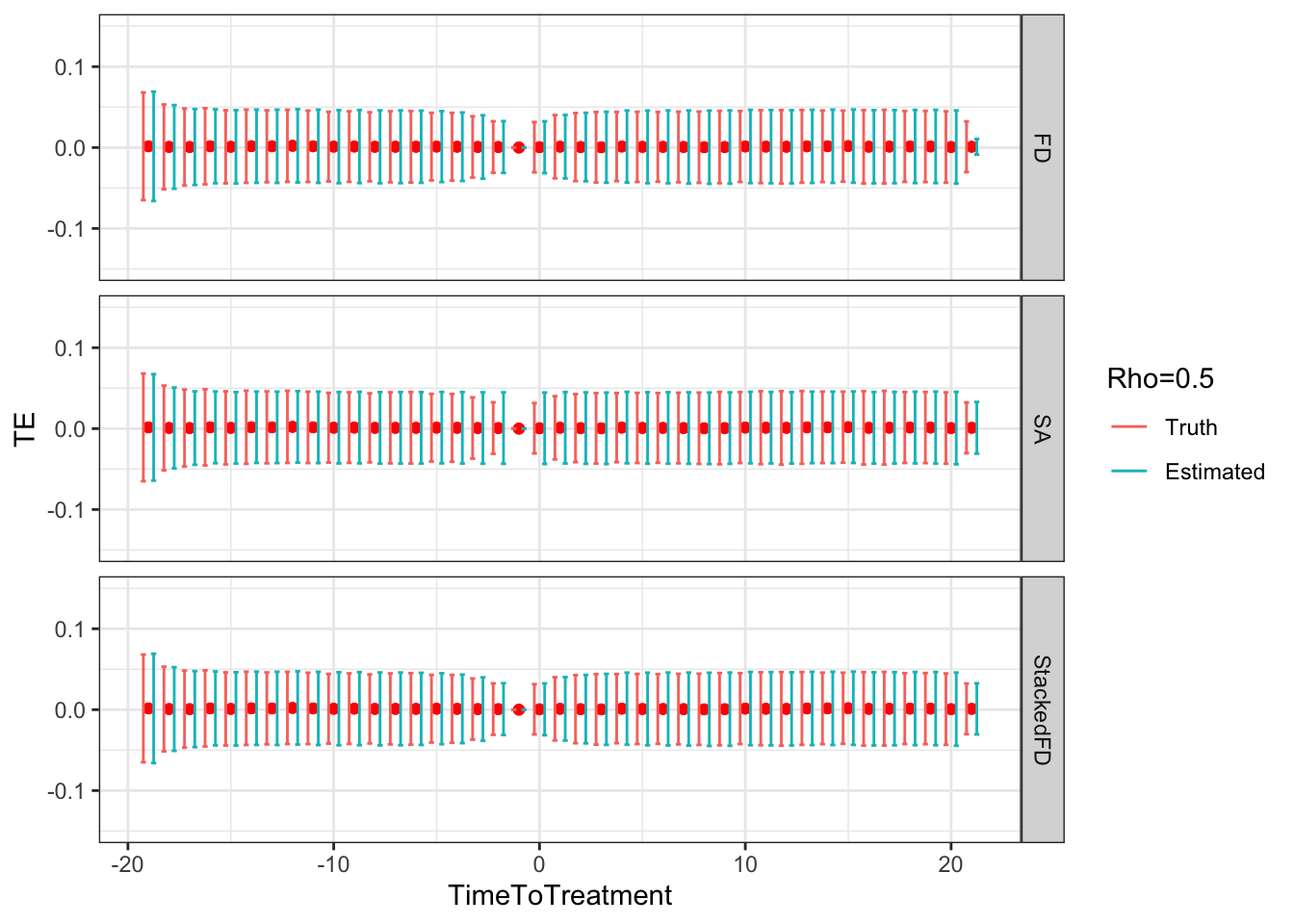
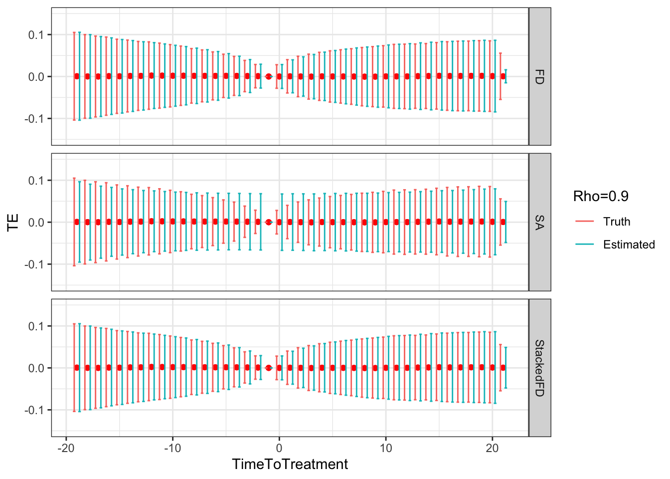
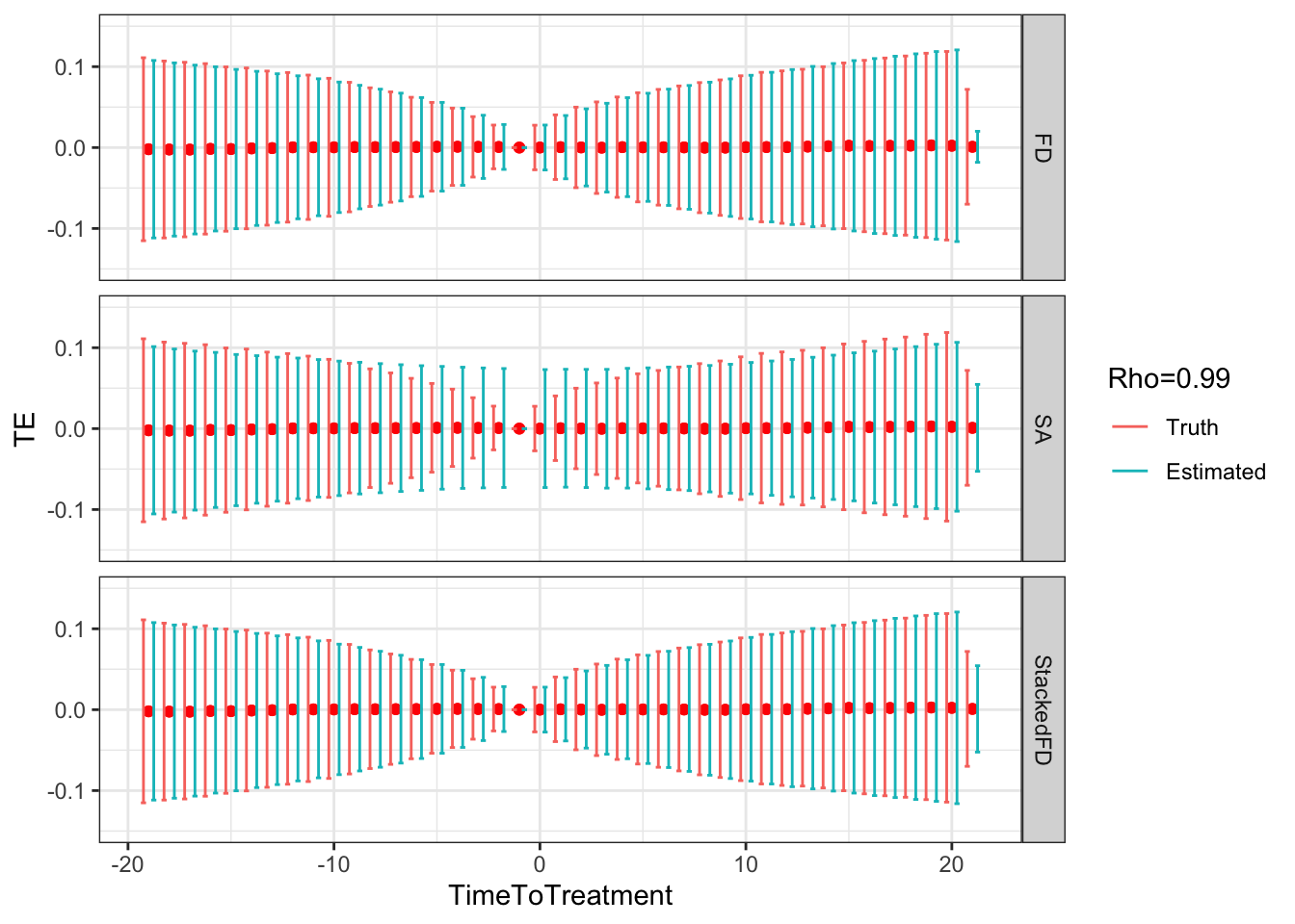
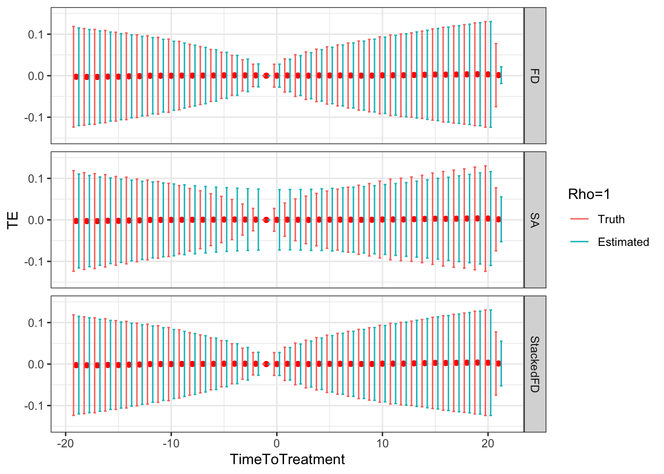
Figure 9.5: DID estimates with increasing temporal autocorrelation in outcomes
Figure 9.5 shows that indeed sampling noise increases with autocorrelation in panel data. For the same sample size of \(N=1000\), the true 99% sampling noise for the average effect of the treatment on the treated estimated by Monte Carlo simulations is equal to:
- 0.07 when \(\rho=0\),
- 0.08 when \(\rho=0.5\),
- 0.14 when \(\rho=0.9\),
- 0.19 when \(\rho=0.99\),
- 0.2 when \(\rho=1\).
The heteroskedasticity-robust estimates of 99% sampling noise for the average effect of the treatment on the treated ignoring autocorrelation are equal to (taking the average estimate of sampling noise over Monte Carlo replications for the the fixest implementation of the Sun and Abraham estimator and for the Stacked First Difference estimator, respectively):
- 0.07 and 0.07 when \(\rho=0\),
- 0.08 and 0.08 when \(\rho=0.5\),
- 0.13 and 0.13 when \(\rho=0.9\),
- 0.14 and 0.14 when \(\rho=0.99\),
- 0.14 and 0.14 when \(\rho=1\).
This means that heteroskedasticity-robust estimates of 99% sampling noise for the average effect of the treatment on the treated ignoring autocorrelation is smaller than the truth, by a factor of (for the the fixest implementation of the Sun and Abraham estimator and for the Stacked First Difference estimator, respectively):
- 1.04 and 1.02 when \(\rho=0\),
- 1.02 and 1.01 when \(\rho=0.5\),
- 0.89 and 0.88 when \(\rho=0.9\),
- 0.76 and 0.75 when \(\rho=0.99\),
- 0.71 and 0.71 when \(\rho=1\).
As true autocorrelation increases, the heteroskedasticity-robust estimator of the sampling noise of the TT parameter increasingly over-estimates true sampling noise. At the same time, the heteroskedasticity-robust \(2\times 2\) estimates of sampling noise underestimate the sampling noise of ATT in a major way. This is because they for now ignore any autocorrelation between \(2\times 2\) estimates as studied in Theorem 4.27.
Remark. An interesting feature of Figure 9.5 is that, when \(\rho>0\), sampling noise decreases as we move closer to to the treatment date and increases as we move away.
Why is that so?
It is due to a combination of our choice of reference period and of the extent of autocorrelation in the error terms.
Indeed, following Theorem 4.25, we know that the sampling noise of each individual \(2\times 2\) estimate depends on the variance of \(Y^0_{i,d+\tau}-Y^0_{i,d-1}\), and thus on the variance of \(U_{i,d+\tau}-U_{i,d-1}\)
Under our \(AR(1)\) model of dynamics of \(U_{i,t}\) and substituting iteratively, we have:
\[\begin{align*} U_{i,d+\tau}-U_{i,d-1} & = \rho^{\tau+1}U_{i,d-1}+\sum_{k=0}^{\tau}\rho^{k}\epsilon_{i,d+\tau-k}-U_{i,d-1}. \end{align*}\]
As a consequence, we have:
\[\begin{align*} \var{U_{i,d+\tau}-U_{i,d-1}} & = (1-\rho^{\tau+1})^2\var{U_{i,d-1}}+\sum_{k=0}^{\tau}\rho^{2k}\sigma^2_{\epsilon}\\ & = (1-\rho^{\tau+1})^2\var{U_{i,d-1}}+\frac{1-\rho^{2(\tau+1)}}{1-\rho^{2}}\sigma^2_{\epsilon}, \end{align*}\]
where the last term in the right hand side of the second equality is valid when \(\rho<1\), and is replaced by \((\tau+1)\sigma^2_{\epsilon}\) when \(\rho=1\). That formula means that when \(\tau\) is close to \(-1\), that is when the estimation period is close to the reference period, the variance of the \(2\times 2\) DID estimate is small. When \(\tau\) increases and the estimation period gets further away from the reference period, the variance of the \(2\times 2\) DID estimate increases. The intuition for this result is that, with autocorrelated error terms, the outcomes of the same individual observed at periods that are close to each other in time are positively correlated, and the first differencing of DID gets rid of part of their influence. In the limit, with perfectly persistent error terms (\(\rho=1\)), the shocks that occur up to the reference period \(d-1\) are completely cancelled (first part of the right hand side of the equation).
Remark. A more unexpected result, is that, when autocorrelation increases, fixest heteroskedasticity-robust estimates of sampling noise using Sun and Abraham estimator overestimate true sampling noise in a major way when treatment and reference periods are close to each other (Method=="SA"), and seems to slighlty underestimate it when the treatment and reference period are far apart.
This is strange because using heteroskedasticity-robust \(2\times 2\) and Stacked First Difference estimates of sampling noise gives a correct estimate of the amount of true sampling noise, irrespective of the level of autocorrelation in the data.
It looks as if the heteroskedasticity-robust estimator of sampling noise in fixest fails at identifying and estimating correctly the heteroskedasticity that takes place across time periods, and instead smooths out the variance over all time periods.
The reason for this behavior lies in how fixest estimates sampling noise.
The feols command in fixest uses a within type of estimator.
As a consequence, it recovers estimates of residuals in levels, not in first difference as with the \(2\times 2\) estimates in First Difference or the Stacked FD estimator.
Therefore, the feols command in fixest does not use the estimator in Theorem 4.25 which involves the residual of the FD estimator, but rather something equivalent to the estimate in Theorem 4.24, with \(Y_{i,t}\) replaced by \(U_{i,t}\).
These two approaches are equivalent when the error terms are independent over time (i.e under Assumption 4.28), but they do not yield the same estimates when the error terms are correlated over time.
Indeed, \(\var{Y_{i,d+\tau}^1-Y_{i,d-1}^0}=\var{Y_{i,d+\tau}^1}+\var{Y_{i,d-1}^0}-2\cov{Y_{i,d+\tau}^1,Y_{i,d-1}^0}\).
When \(\cov{Y_{i,d+\tau}^1,Y_{i,d-1}^0}>0\), the variance of the difference is smaller than the sum of the variances of each components, and thus the estimate of samling noise based on the FD estimators is going to be smaller than the one based on the within estimator (as in fixest).
It is less clear why fixest heteroskedasticity-robust estimates of sampling noise using Sun and Abraham estimator slighlty underestimates sampling noise when the treatment and reference period are far apart.
This is an open question at the time of writing.
9.2.2 Design effect in panel data
Let us now derive an estimate of the design effect in panel data.
9.2.2.1 Design effect for \(2\times 2\) DID estimates
Autocorrelation of error terms over time does not affect the estimates of sampling noise for the individual \(2\times 2\) DID estimates in panel data based on the First-Difference transformation. Indeed, Theorem 4.25 only rests on the fact that outcomes are independent over space, not over time (Assumption 4.15). This is confirmed by the simulations in Figure 9.5: when \(\rho>0\), and thus there is autocorrelation between outcomes over time, the estimates of sampling noise of the individual \(2\times 2\) DID estimates based on Theorem 4.25 (for the \(2\times 2\) First Difference and Stacked First Difference estimators) are correct. The reason is that the \(2\times 2\) First Difference estimators are purely cross-sectional: they do not involve observations from several periods. All of that is taken into account in the differencing part. As a consequence, the validity of the estimates of sampling noise of the \(2\times 2\) DID estimates based on Theorem 4.25 are valid under any type of autocorrelation, which makes them extremely attractive.
In contrast, \(2\times 2\) DID estimates in panel data that are not based on the First Difference transformation, but rather on the within transformation, such as the ones obtained using the feols command of the fixest package, require an absence of temporal autocorrelation to be valid.
They will overestimate the extent of sampling noise when error terms are positively correlated over time, and they will underestimate sampling noise when error terms are negatively correlated over time.
9.2.2.2 Design effect for the Average Treatment Effect on the Treated
Estimates of sampling noise for the Average Treatment Effect on the Treated will always be affected by temporal auto-correlation of the error terms, even when the estimates of sampling noise for the individual \(2\times 2\) DID estimates is not. The intuition for why is that, when error terms are correlated over time, individual \(2\times 2\) DID estimates are more correlated with each other than what Theorem 4.27 would suggest. If they are more correlated, then the variance of their weighted average increases, since it is more likely that two individual \(2\times 2\) DID estimates look alike than what we would have expected under Assumption 4.28. Let’s see how the sampling noise of the Average Treatment Effect on the Treated changes when relaxing Assumption 4.28.
Hypothesis 9.2 (AR(1) autocorrelation and i.i.d. sampling in panel data) We assume that potential outcomes are generated as follows:
\[\begin{align*} Y^0_{i,t} & = \mu_i + \delta_t + U^0_{i,t}\\ Y^1_{i,t} & = \mu_i + \delta_t + \bar{\alpha} +\eta_{i,t} + U^0_{i,t}\\ U^0_{i,t} & = \rho U^0_{i,t-1} + \epsilon_{i,t}, \end{align*}\]
with \(\esp{U^0_{i,t}}=\esp{\eta_{i,t}}=0\), \(\forall t\), \(\esp{U^0_{i,t}|D_i}=0\), \(\forall t\) and:
\[\begin{align*} \forall i,j\leq N\text{, }\forall t,t'\leq T\text{, with either }i\neq j \text{ or } t\neq t' & (\epsilon_{i,t},\eta_{i,t},D_i)\Ind(\epsilon_{j,t'},\eta_{j,t'},D_j),\\ & (\epsilon_{i,t},\eta_{i,t},D_i)\&(\epsilon_{j,t'},\eta_{j,t'},D_j)\sim F_{\epsilon,\eta,D}. \end{align*}\]
We also assume that \(U^0_{i,t}\Ind\epsilon_{j,t'},\eta_{j,t'}\), \(\forall i,j\leq N\text{, }\forall t,t'\leq T\).
Remark. Assumption 9.2 is less restrictive than Assumption 4.28: it allows for error terms for the same unit \(i\) to be correlated over time through an AR(1) process. Assumption 9.2 nevertheless still imposes than treatment effects are not autocorrelated over time, which is still pretty restrictive.
Theorem 9.2 (Asymptotic Distribution of Treatment of the Treated Estimated Using Sun and Abraham Estimator in Panel Data with AR(1) Error Terms) Under Assumptions 4.12, 4.13, 4.14, 9.2 and 4.16, and with panel data containing a total of \(N\) units observed over \(T\) time periods, we have:
\[\begin{align*} \sqrt{N}(\hat\Delta^{Y}_{TT_{SA}}(k)-\Delta^{Y}_{TT_{SA}}(k)) & \stackrel{d}{\rightarrow} \mathcal{N}\left(0,\sum_d\sum_{\tau}V_P(\hat\beta^{SA}_{d,\tau})(w^k(d,d-1,\tau,\infty))^2\right.\\ & \phantom{\stackrel{d}{\rightarrow}}\left.+\sum_{d}\sum_{d'}\sum_{\tau}\sum_{\tau'\neq\tau} \text{Cov}_P(\hat\beta^{SA}_{d,\tau},\hat\beta^{SA}_{d',\tau'})w^k(d,d-1,\tau,\infty)w^k(d',d'-1,\tau',\infty)\right), \end{align*}\]
where:
\[\begin{align*} V_P(\hat\beta^{SA}_{d,\tau}) & =\frac{1}{p^{d,\infty}}\left(\frac{\var{Y_{i,d+\tau}^1-Y_{i,d-1}^0|D_i=d}}{p^{d,\infty}_D}+\frac{\var{Y_{i,d+\tau}^0-Y_{i,d-1}^0|D_i=\infty}}{1-p^{d,\infty}_D}\right)\\ \text{Cov}_P(\hat\beta^{SA}_{d,\tau},\hat\beta^{SA}_{d',\tau'}) & =\frac{1}{p^{d,\infty}}\left[\frac{\esp{\Delta\epsilon^{d,\tau}_i\Delta\epsilon^{d',\tau'}_i|D_i=\infty}}{1-p^{d,\infty}_D}+\frac{\esp{\Delta\epsilon^{d,\tau}_i\Delta\epsilon^{d',\tau'}_i|D_i=d}}{p^{d,\infty}_D}\right] \text{ when } d=d'\\ & = \frac{\esp{\Delta\epsilon^{d,\tau}_i\Delta\epsilon^{d',\tau'}_i|D_i=d}}{p^{d',\infty}(1-p^{d',\infty}_D)} \text{ when } d\neq d', \end{align*}\]
with \(p^{d,\infty}=\Pr(D_i=d\cup D_i=\infty)\) and \(p^{d,\infty}_D=\Pr(D_i=d|D_i=d\cup D_i=\infty)\).
Proof. See Section A.5.2.
9.2.3 Estimating sampling noise in panel data with autocorrelated error terms
We are now equipped to estimate sampling noise in panel data with autocorrelated error terms. As in the case of spatial autocorrelation, the solutions involve using the plug-in estimator based on Theorem 9.2, using cluster-robust standard errors, using Feasible Generalized Least Squares, the bootstrap and randomization inference.
9.2.3.1 Using the plug-in estimator
Although a little bit tedious, it is possible to estimate each component of the plug-in formula in Theorem 9.2, whose details can be found in Section A.5.2. We need mostly to estimate \(\rho\), by regressing \(\hat{U}^0_{i,t}\) on \(\hat{U}^0_{i,t-1}\). We then need to estimate the variance terms. This is left as an exercise.
9.2.3.2 Using Feasible Generalized Least Squares
It is possible to build the matrix \(\hat{\Omega}_{GLS}=\hatesp{UU'|X}\) under Assumption 4.28. It is a block diagonal matrix, with all blocks being the observations over time of the same unit in the panel. The covariance terms depend on \(\hat\rho\) and the variance of \(\hat{U}^0_{i,t}\) and \(\eta_{i,t}\). Estimating the terms in this matrix is left as an exercise. CLuster-robust FGLS estimates are also feasible, obviously.
9.2.3.3 Using Cluster-Robust Standard Errors
As in the spatial clustering case, it is possible to use a cluster robust covariance matrix in panel data with autocorrelated error terms.
For the within estimator, the formula can be derived in the same way, except with clusters being the groups of observations belonging to the same unit observed over time.
Estimating this formula can be done with either the sandwich package or the cluster option in the fixest package.
Here, I want to introduce an alternative approach, which is going to make our lives much easier when correlation between error terms is going to be richer and more complex. This approach is due to Leung (2020) and it generalizes cluster-robust covariance matrices to a much broader set of cases while retaining the interpretability of the cluster-robust standard errors. Leung’s estimator of the variance of the OLS estimator is as follows: \(\hatvar{\hat{\Theta}_{OLS,Leung}}=(X'X)^{-1}\hat{\mathcal{M}}'G\hat{\mathcal{M}}(X'X)^{-1}\), where \(\hat{\mathcal{M}}=(X_1\hat{\epsilon}_1,\dots,X_N\hat{\epsilon}_N)'\), with \(\hat{\epsilon}\) the vector of regression residuals and \(X_k\) the vector of covariates for observation \(k\), and \(G\) is a matrix indicating which observations are correlated with each other. In the case of temporal autocorrelation, \(G_{i,j}\) takes value \(1\) when observations \(i\) and \(j\) in the dataset belong to the same unit and zero otherwise.
Example 9.8 Let’s see how this all works in our example.
We actually already introduced the cluster option in the original Monte Carlo simulation functions.
Extending our simulations to clustering is therefore straightfoward.
# true simulations
Nsim <- 1000
sf.simuls.Cluster.DID.Temporal.grid.rho <- sf.Cluster.MonteCarlo.DID.Grid(grid.rho=grid.rho.test,Nsim=Nsim,N=1000,K=40,k=20,param=param.basic,cluster='Temporal',ncpus=8)
Let us now plot the resulting estimates:
# prepapring data
sf.simuls.Cluster.DID.Temporal.grid.rho <- sf.simuls.Cluster.DID.Temporal.grid.rho %>%
                                    mutate(
                                      TimeToTreatment = case_when(
                                        TimeToTreatment == "99" ~ 21,
                                        TRUE ~ TimeToTreatment
                                      ),
                                      Rho = factor(Rho,levels=as.character(grid.rho.test))
                                    ) %>%
                                    pivot_longer(cols=SdTE:MeanSeTE,names_to = "Type",values_to="SeEstim") %>%
                                    mutate(
                                      Type = case_when(
                                        Type == "MeanSeTE" ~ "Estimated",
                                        Type == "SdTE" ~ "Truth",
                                        TRUE ~ ""
                                      ),
                                      Type = factor(Type,levels=c("Truth","Estimated"))
                                    ) #%>%
                                    #pivot_wider(names_from = "Method",values_from = c('TE','SeEstim'))

ggplot(sf.simuls.Cluster.DID.Temporal.grid.rho %>% filter(Rho==0),aes(x=TimeToTreatment,y=TE,group=Type,color=Type))+
#  geom_pointrange(aes(ymin=TE-1.96*SeEstim,ymax=TE+1.96*SeEstim),position=position_dodge(1))+
  geom_point(color='red') +
  geom_errorbar(aes(ymin=TE-1.96*SeEstim,ymax=TE+1.96*SeEstim,color=Type,group=Type),position=position_dodge(1),width=0.5)+
  coord_cartesian(ylim=c(-0.15,0.15))+
  scale_color_discrete(name='Rho=0')+
  theme_bw()+
  facet_grid(Method~.)
ggplot(sf.simuls.Cluster.DID.Temporal.grid.rho %>% filter(Rho==0.5),aes(x=TimeToTreatment,y=TE,group=Type,color=Type))+
#  geom_pointrange(aes(ymin=TE-1.96*SeEstim,ymax=TE+1.96*SeEstim),position=position_dodge(1))+
  geom_point(color='red') +
  geom_errorbar(aes(ymin=TE-1.96*SeEstim,ymax=TE+1.96*SeEstim,color=Type,group=Type),position=position_dodge(1),width=0.5)+
  coord_cartesian(ylim=c(-0.15,0.15))+
  scale_color_discrete(name='Rho=0.5')+
  theme_bw()+
  facet_grid(Method~.)
ggplot(sf.simuls.Cluster.DID.Temporal.grid.rho %>% filter(Rho==0.9),aes(x=TimeToTreatment,y=TE,group=Type,color=Type))+
#  geom_pointrange(aes(ymin=TE-1.96*SeEstim,ymax=TE+1.96*SeEstim),position=position_dodge(1))+
  geom_point(color='red') +
  geom_errorbar(aes(ymin=TE-1.96*SeEstim,ymax=TE+1.96*SeEstim,color=Type,group=Type),position=position_dodge(1),width=0.5)+
  coord_cartesian(ylim=c(-0.15,0.15))+
  scale_color_discrete(name='Rho=0.9')+
  theme_bw()+
  facet_grid(Method~.)
ggplot(sf.simuls.Cluster.DID.Temporal.grid.rho %>% filter(Rho==0.99),aes(x=TimeToTreatment,y=TE,group=Type,color=Type))+
#  geom_pointrange(aes(ymin=TE-1.96*SeEstim,ymax=TE+1.96*SeEstim),position=position_dodge(1))+
  geom_point(color='red') +
  geom_errorbar(aes(ymin=TE-1.96*SeEstim,ymax=TE+1.96*SeEstim,color=Type,group=Type),position=position_dodge(1),width=0.5)+
  coord_cartesian(ylim=c(-0.15,0.15))+
  scale_color_discrete(name='Rho=0.99')+
  theme_bw()+
  facet_grid(Method~.)
ggplot(sf.simuls.Cluster.DID.Temporal.grid.rho %>% filter(Rho==1),aes(x=TimeToTreatment,y=TE,group=Type,color=Type))+
#  geom_pointrange(aes(ymin=TE-1.96*SeEstim,ymax=TE+1.96*SeEstim),position=position_dodge(1))+
  geom_point(color='red') +
  geom_errorbar(aes(ymin=TE-1.96*SeEstim,ymax=TE+1.96*SeEstim,color=Type,group=Type),position=position_dodge(1),width=0.5)+
  coord_cartesian(ylim=c(-0.15,0.15))+
  scale_color_discrete(name='Rho=1')+
  theme_bw()+
  facet_grid(Method~.)

# ggplot(sf.simuls.Cluster.DID.grid.rho,aes(x=TimeToTreatment,y=TE_FD,group=Type,color=Type))+
# #  geom_pointrange(aes(ymin=TE-1.96*SeEstim,ymax=TE+1.96*SeEstim),position=position_dodge(1))+
#   geom_point(color='red') +
#   geom_errorbar(aes(ymin=TE_FD-1.96*SeEstim_FD,ymax=TE_FD+1.96*SeEstim_FD,color=Type,group=Type),position=position_dodge(1),width=0.2)+
#   geom_errorbar(aes(ymin=TE_SA-1.96*SeEstim_SA,ymax=TE_SA+1.96*SeEstim_SA,color=Type,group=Type),position=position_dodge(1),width=0.5)+
#   geom_errorbar(aes(ymin=TE_StackedFD-1.96*SeEstim_StackedFD,ymax=TE_StackedFD+1.96*SeEstim_StackedFD,color=Type,group=Type),position=position_dodge(1),width=0.9)+
#   theme_bw()+
#   facet_grid(Rho~.)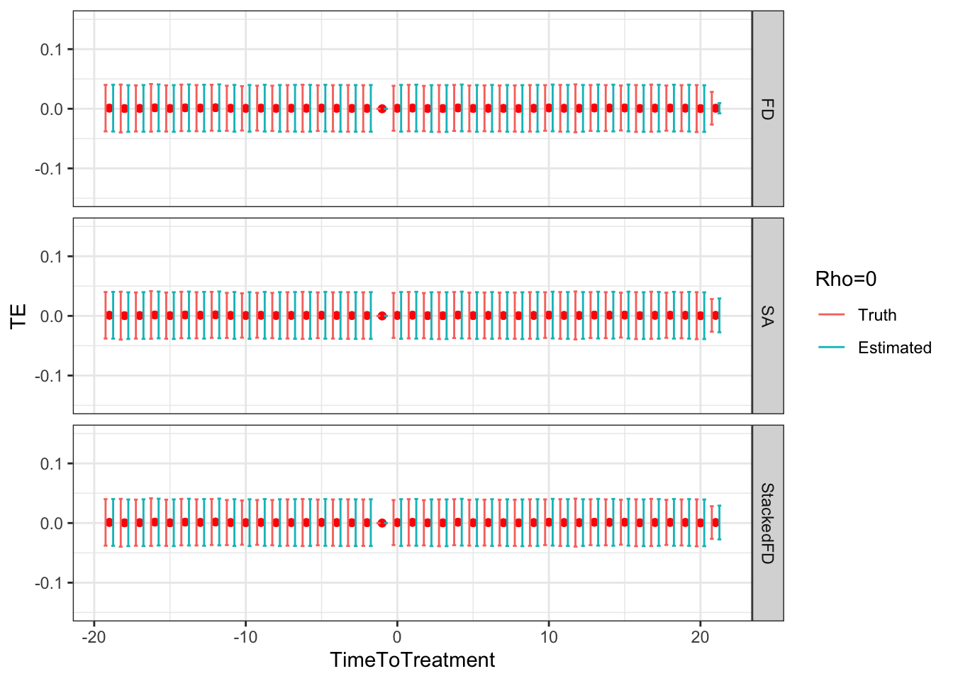
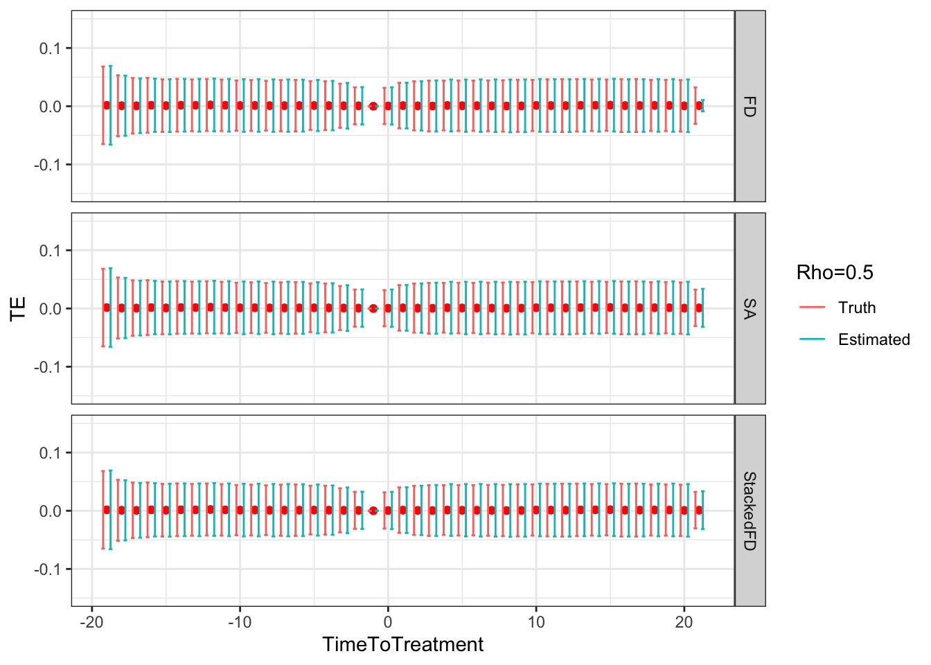
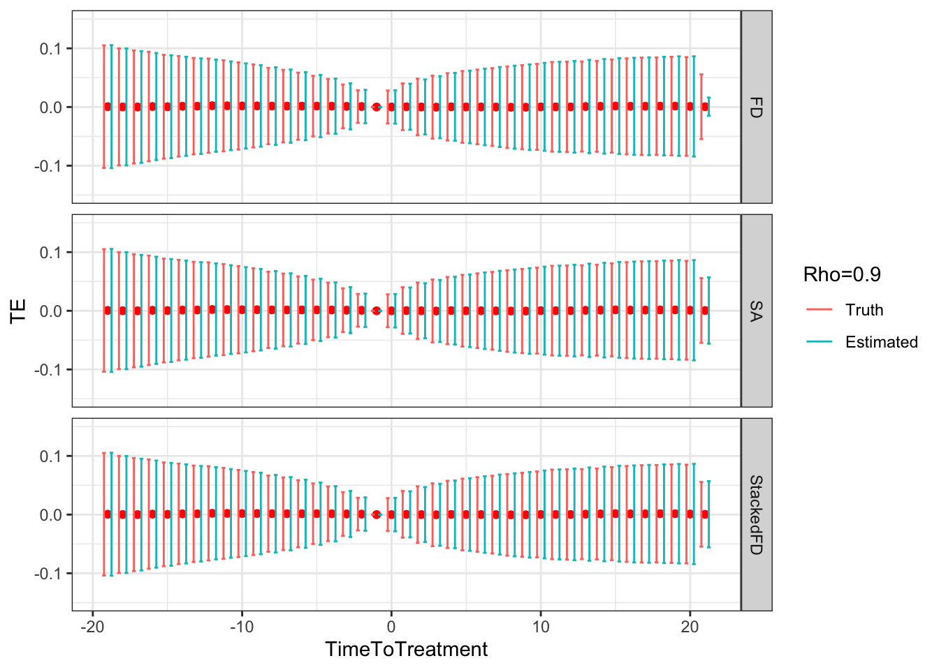
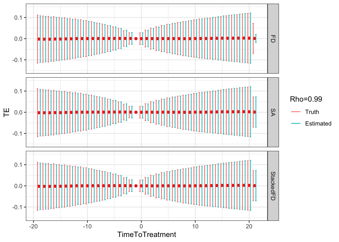
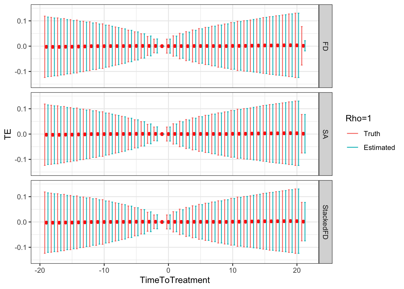
Figure 9.6: Clustered DID estimates of sampling noise with increasing temporal autocorrelation in outcomes
Two results appear clearly on Figure 9.6:
- The estimates of sampling noise for the ATT are now correct both with the Sun and Abraham estimator implemented with
fixestand theclusteroption and with the Stacked First Difference estimator implemented with the Leung covariance matric estimator. It even seems that the estimates of sampling noise are slightly too large with respect to the results of the simulations, but overall, the result is pretty good. - The estimates of sampling noise for the individual \(2\times 2\) DID estimates estimated with the Sun and Abraham estimator implemented with
fixestand theclusteroption have now a correct estimate of sampling noise. Theclusteroption is here critical to take into account the fact that the error terms that belong to the same unit observed at different time periods are negatively autocorrelated. We should therefore always use the theclusteroption when using the Sun and Abraham estimator implemented withfixest.
9.2.3.4 Using the Bootstrap
The bootstrap can be used exactly in the same way as we have seen for clustering in RCTs in Section 9.1. The only difference is that clusters here are units and therefore one samples with replacement among units, and includes all the observations of the same unit over time when it has been sampled. Implementation is left as an exercise.
9.2.3.5 Using Randomization Inference
Similarly as in Section 9.1, we can also use randomization inference. We again have to build potential outcomes under the assumed null, both before and after the various treatment dates, and to allocate the treatment date at random across units, among the dates that actually exist in the sample, respecting their actual proportions. Implementation is left as an exercise.
9.3 Spatial correlation
Clusters are a very peculiar form of autocorrelation: it is identical for all members of the cluster and stops abruptly at the border of the cluster. Sometimes, the treatment and the outcomes of interest are correlated across units in a less crude way than through clusters. For example, it might very well be that observations are correlated more smoothly across space, such as for example neighboring observations, that is observations that are close in space, sharing unobserved influences both for their outcomes and for their treatment status. Does this smoother form of spatial autocorrelation matter for sampling noise? Do we have to adapt our estimators of sampling noise accordingly? If yes, when and how? These are the questions we are going to examine here.
9.3.1 An example
We are going to generate data with spatially autocorrelated error terms. We are going to denote \(W\) our matrix of spatial influence. \(W\) is a square matrix of size \(N\times N\), where \(N\) is sample size. Row \(i\) of \(W\) is a vector of weights \(w_{i,j}\) between zero and one, which sum to one (\(\sum_{j=1}^Nw_{i,j}=1\)), and which correspond to the influence each observation \(j\) has on observation \(i\). \(W\) has a diagonal of zeroes, since each observation does not influence itself. We can thus write, in matrix form:
\[\begin{align*} U & = \rho WU + \epsilon \end{align*}\]
where \(U\) is the vector of all autocorrelated error terms for all \(N\) observations and \(\epsilon\) is an i.i.d. random vector of the same size. In order to build \(U\), we can make use of the fact that:
\[\begin{align*} U & = (I_N-\rho W)^{-1}\epsilon, \end{align*}\]
where \(I_N\) is the identity matrix of size \(N\). For assignment to the treatment, we are going to use an independent set of random variables that exhibits the same pattern of spatial autocorrelation:
\[\begin{align*} V & = (I_N-\rho W)^{-1}\eta\\ D_i & = \uns{V_i\geq0}, \end{align*}\]
where \(\eta\) is a vector of i.i.d. shocks independent from \(\epsilon\).
In order to generate this spatial process, we first need spatial data.
For that, we are going to draw coordinates randomly in latitudes and longitudes, and define distances among the resulting points.
I’m going to choose points within the French territory, between 46 and 49 degress of latitude and 0 and 3 degrees of longitude.
I’m using the sf package to then convert these coordinates to a map.
set.seed(12345)
SpatialData <- data.frame(id=1:1000,latitude=runif(1000,49.8,51),longitude=runif(1000,1.8,2.8)) %>%
        st_as_sf(.,coords=c('longitude','latitude'),crs=4326)

# extracting coordinates from `sf` object for later uses
SpatialData <-SpatialData %>%
        mutate(
          latitude = st_coordinates(SpatialData)[,2],
          longitude = st_coordinates(SpatialData)[,1]
        )
Let us plot these data:
# Map of France
FranceMap <- st_as_sf(maps::map("france",plot=FALSE,fill=TRUE,crs=4326))

# Map
ggplot(data=FranceMap,fill="transparent") +
  geom_sf(fill="transparent")+
  geom_sf(data=SpatialData)+
#  coord_sf(xlim = c(-5, 8), ylim = c(48,51))+
  coord_sf(xlim = c(1,3), ylim = c(49.5,51))+
  theme_bw()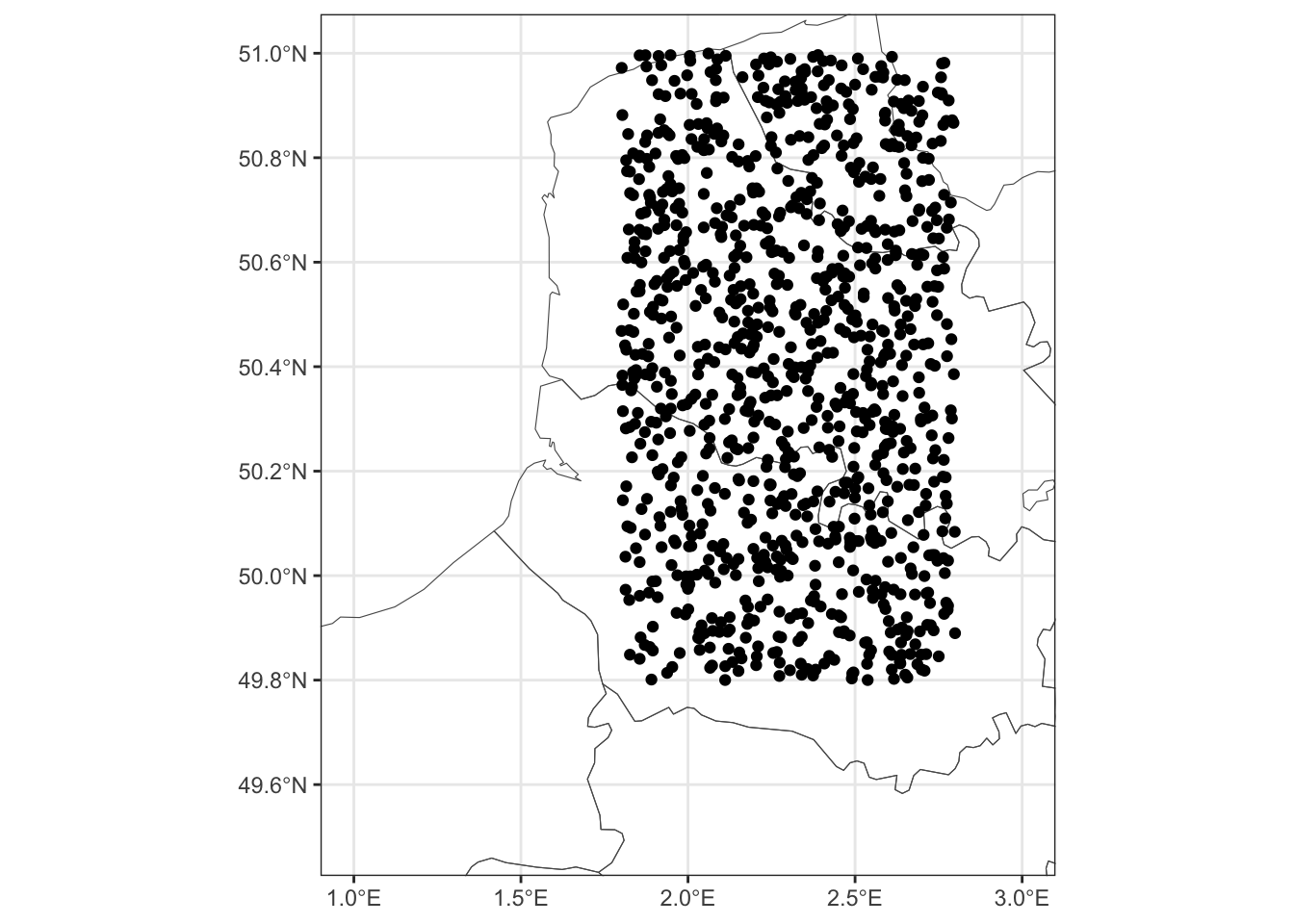
Figure 9.7: Map of our sample points
Let us now compute the distance between all of these points in kilometers:
Let us now take 10 kilometers as a boundary to define influence.
# distance (in km)
dist <- 10
# computation of the discrete influence matrix
DistanceMatrixDiscrete <- as.numeric(DistanceMatrix)
DistanceMatrixDiscrete[DistanceMatrixDiscrete<=dist] <-  1
DistanceMatrixDiscrete[DistanceMatrixDiscrete>dist] <-  0
# the diagonal terms are all zeroes, since we want close neighbors and not egos to be ones
DistanceMatrixDiscrete[as.numeric(DistanceMatrix)==0] <-  0
# forming a sparse matrix
DistanceMatrixDiscrete <- Matrix(data=DistanceMatrixDiscrete,nrow=1000,ncol=1000,byrow=TRUE,sparse=TRUE)

# for later uses, same but with 20km
# distance (in km)
dist <- 20
# computation of the discrete influence matrix
DistanceMatrixDiscrete20 <- as.numeric(DistanceMatrix)
DistanceMatrixDiscrete20[DistanceMatrixDiscrete20<=dist] <-  1
DistanceMatrixDiscrete20[DistanceMatrixDiscrete20>dist] <-  0
# the diagonal terms are all zeroes, since we want close neighbors and not egos to be ones
DistanceMatrixDiscrete20[as.numeric(DistanceMatrix)==0] <-  0
# forming a sparse matrix
DistanceMatrixDiscrete20 <- Matrix(data=DistanceMatrixDiscrete20,nrow=1000,ncol=1000,byrow=TRUE,sparse=TRUE)
Let us now compute the sum of the entries in each row, and divide each row by this sum, to normalize each neighbor by the number of neighbors and obtain weights that sum to one in each row.
DistanceMatrixDiscreteRowSum <- 1/rowSums(DistanceMatrixDiscrete)
DistanceMatrixDiscreteWeights <- DistanceMatrixDiscreteRowSum*DistanceMatrixDiscrete
# same with 20 km for later uses
DistanceMatrixDiscreteRowSum20 <- 1/rowSums(DistanceMatrixDiscrete20)
DistanceMatrixDiscreteWeights20 <- DistanceMatrixDiscreteRowSum20*DistanceMatrixDiscrete20
Now, in order to compute autocorrelated error terms from i.i.d. errors, we need to form the matrix \((I_N-\rho W)^{-1}\), where \(I_N\) is the identity matrix of size \(N\) and \(W\) our spatial influence matrix with rows summing to one, and \(\rho\) the spatial autocorrelation coefficient.
Let us finally generate our autocorrelated error terms \(U=(I_N-\rho W)^{-1}\epsilon\), where \(\epsilon\) is a vector of i.i.d. shocks:
set.seed(1234)
epsilon <- rnorm(n=1000,mean=0,sd=sqrt(param['sigma2epsilon']))
U <- SpatialInfluenceMatrix%*%epsilon
# Spatially lagged error term
SLU <- DistanceMatrixDiscreteWeights%*%U
Let us now compute the spatial autocorrelation among the error terms in this dataset. This is done using Moran’s \(I\) statistic, which is defined as follows:
\[\begin{align*} I & = \frac{N\sum_i\sum{j\neq i}w_{i,j}(x_i-\bar{x})(x_j-\bar{x})}{\sum_i\sum{j\neq i}w_{i,j}\sum_i\sum{i\neq j}(x_i-\bar{x})^2}, \end{align*}\]
where \(w_{i,j}\) is the element of the \(i\) line and the \(j\) column in the spatial weighting matrix \(W\). Moran’s \(I\) is the correlation between \(x_i\) and its spatially lagged value. As a result, it can be estimated using OLS and it can be represented as a matrix product, when the \(W\) matrix is row normalised:
\[\begin{align*} I & = \frac{z'Wz}{z'z}, \end{align*}\]
where \(z\) is the vector of all observations \(x_i-\bar{x}\). Let us first look at the correlation between \(U\) and its spatially lagged values \(WU\):
# preparing data
SpatialData$U <- as.numeric(U)
SpatialData$SLU <- as.numeric(SLU)

# plot
ggplot(SpatialData,aes(U,SLU)) +
  geom_point() +
  geom_smooth(method='lm') +
  theme_bw()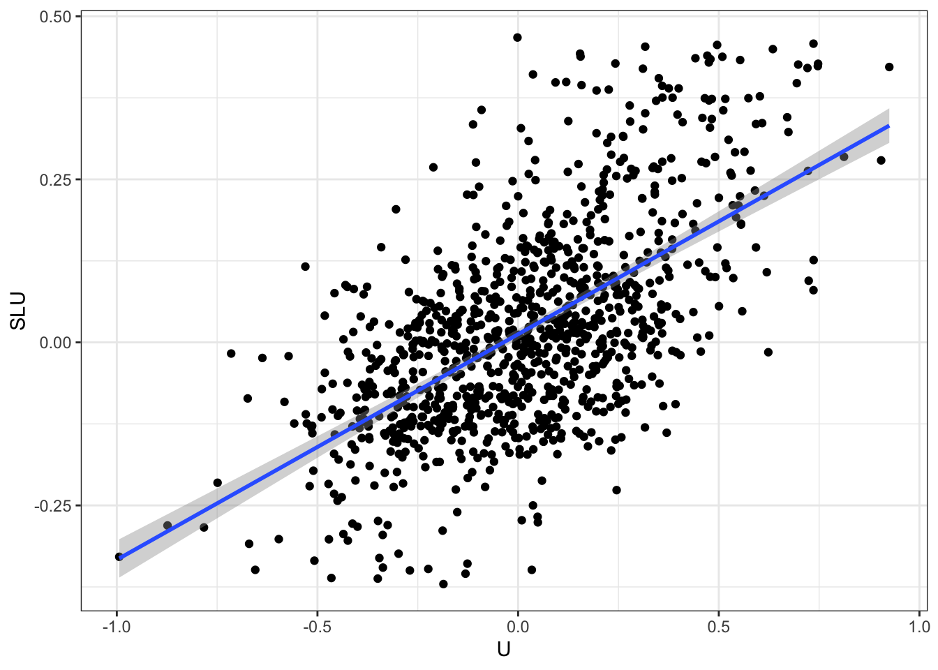
Figure 9.8: Moran’s plot
Let us now compute Moran’s \(I\):
# using regression
MoranReg <- lm(SLU~-1+U,data=SpatialData)
# using matrix notation
MoranMat <- (t(U)%*%DistanceMatrixDiscreteWeights%*%U)/(t(U)%*%U)
In this data, Moran’s \(I\) is equal to 0.35, which is testament to non-trivial spatial autocorrelation. Let us now simulate a process allocating a binary treatment randomly, but with a process that is going to be spatially correlated with the same contiguity matrix as the one used for \(U\):
set.seed(12345)
eta <- rnorm(n=1000,mean=0,sd=sqrt(param['sigma2epsilon']))
SpatialData$SpatialEta <- as.numeric(SpatialInfluenceMatrix%*%eta)
# allocating the treatment
SpatialData <- SpatialData %>%
          mutate(
            Ds = case_when(
                      SpatialEta>0 ~ 1,
                      TRUE ~ 0)
          )
We can now try to visualize what the data looks like, and especially the level of spatial autocorrelation, by mapping the spatial conditional expectation of the two variables of interest.
For that, I am going to use the btb package in R, which has a very nice function to compute spatial conditional expectations: btb_smooth.
Because some of the results I obtain with btb are somewhat strange, I also use the spatstat package and its function markmean.
# with btb
# dataset with X and Y coordinates
# I use the Universal Mercator projection zone 31N, which corresponds to the North of France, and whose EPSG identity is 32631
xy.SpatialData <- SpatialData %>%
                  st_transform(crs=32631) %>%
                  cbind(st_coordinates(SpatialData)) %>%
#                  select(-geometry) %>%
                  relocate(Y) %>%
                  relocate(X) %>%
                  rename(
                    x=X,
                    y=Y
                  )

# choosing parameters
# grid size (in m)
grid.size <- 5000
# bandwidth (in m)
bandwith.radius <- 10000
# estimating spatial conditional expectation
dfSpatialCondExp <- btb::btb_smooth(xy.SpatialData,iCellSize=grid.size,iBandwidth=bandwith.radius,sEPSG="4326") %>%
                    st_transform(4326) %>%
                    st_as_sf()

# with spatstat
range <- owin(xrange=c(min(xy.SpatialData$x),max(xy.SpatialData$x)),yrange=c(min(xy.SpatialData$y),max(xy.SpatialData$y)))
# U
xy.SpatialData.U.ppp <- ppp(xy.SpatialData$x,xy.SpatialData$y,window=range,marks=xy.SpatialData$U)
# smoothing
dfSpatialCondExp.U.ppp <- markmean(xy.SpatialData.U.ppp)
# Ds
xy.SpatialData.Ds.ppp <- ppp(xy.SpatialData$x,xy.SpatialData$y,window=range,marks=xy.SpatialData$Ds)
# smoothing
dfSpatialCondExp.Ds.ppp <- markmean(xy.SpatialData.Ds.ppp)
Let us now plot the resulting maps:
# with btb
cartography::choroLayer(dfSpatialCondExp, var = "U", nclass = 5, method = "fisher-jenks", border = NA, legend.pos = "topright", legend.title.txt ="U")
cartography::choroLayer(dfSpatialCondExp, var = "Ds", nclass = 5, method = "fisher-jenks", border = NA, legend.pos = "topright", legend.title.txt ="Ds")
# with spatstat
plot(dfSpatialCondExp.U.ppp,axes=T,main='U')
plot(dfSpatialCondExp.Ds.ppp,axes=T,main='Ds')
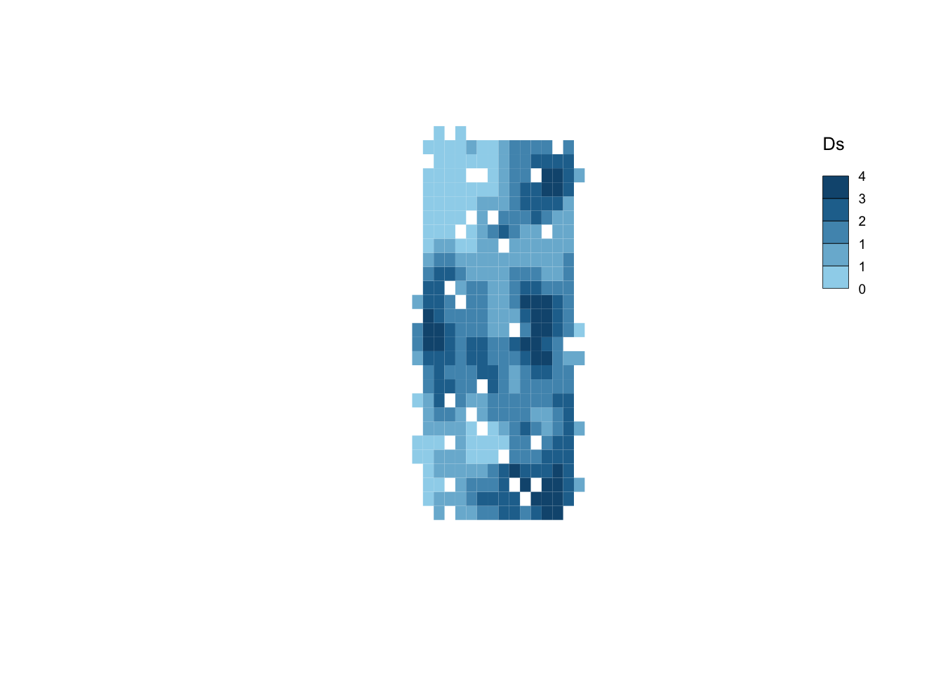
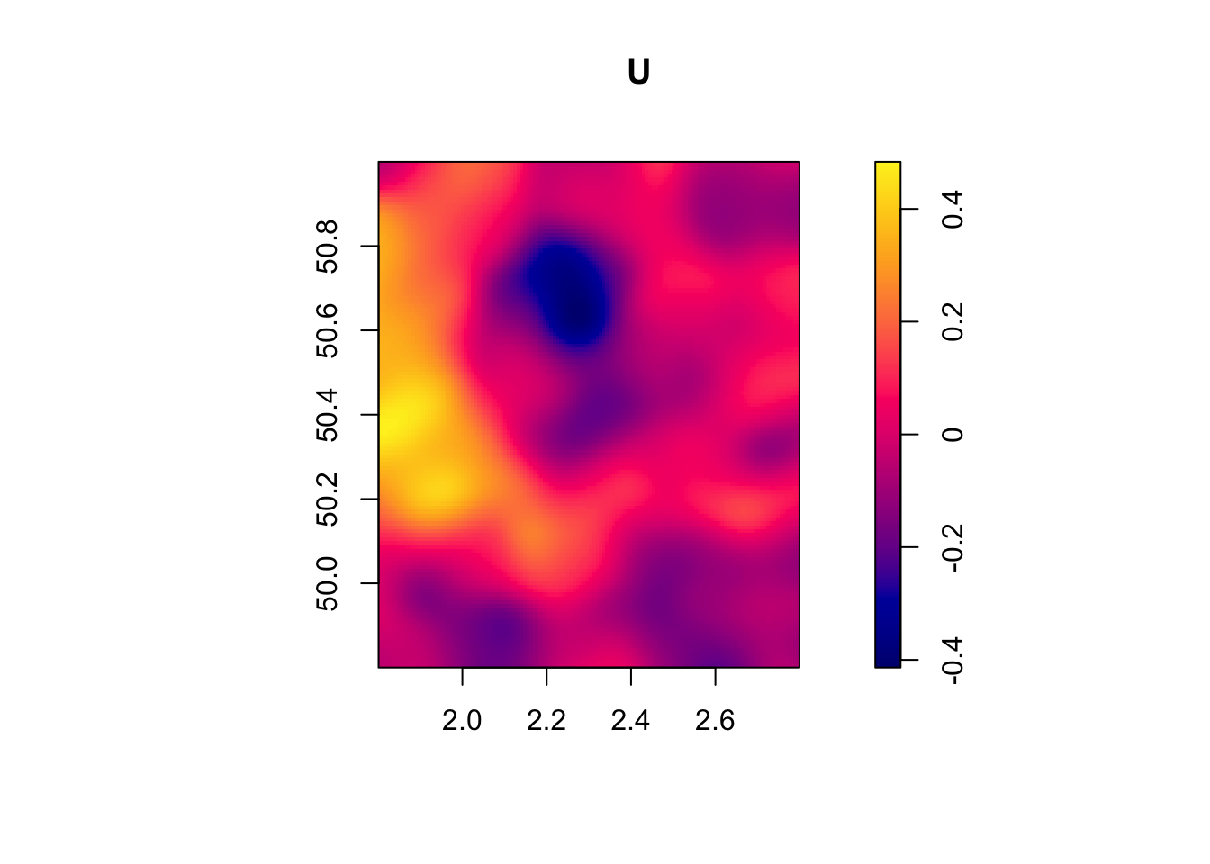
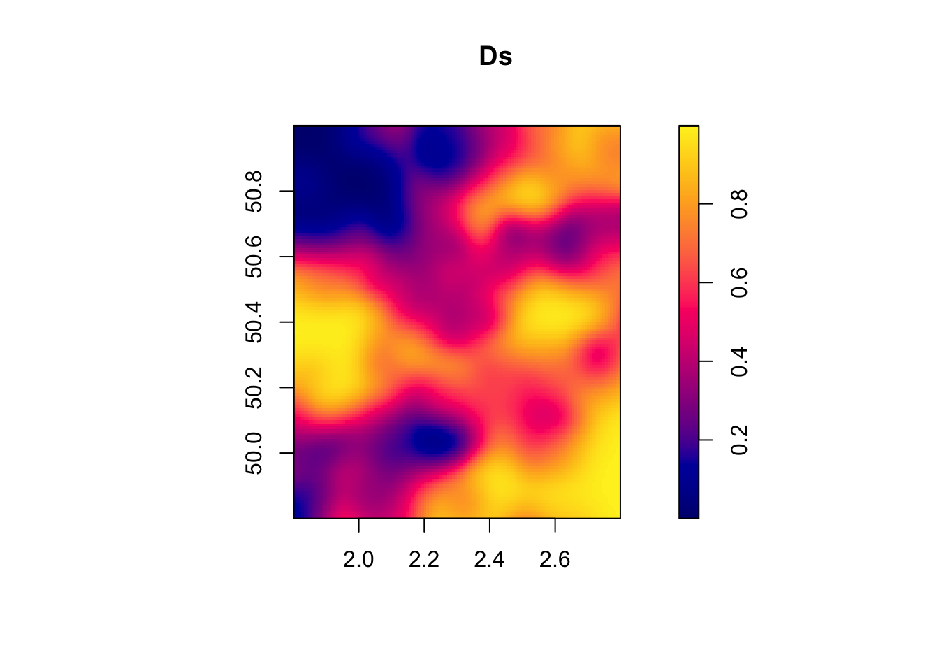
Figure 9.9: Spatial correlation
We can see on the maps that there are clear signs of spatial autocorrelation both in the \(U_i\) variable and in the \(D_i\) variable.
On the btb plots, each pixels has edges of 5km.
The autocorrelation patterns seem larger than that, reaching 15 to 20 km.
On the spatstat plots, units are in meters, meaning that each tick mark measures 20km.
It seems that this is an adequate scale to describe the amount of spatial autocorrelation in the data.
Note finally that the prediction of \(D_i\) obtained with btb is weird, since it is not comprised between 0 and 1, while the one obtained using spatstat makes a lot of sense.
They both offer the same overall picture though: there is substantial spatial autocorrelation in this data.
We finally can run a regression of the outcome \(U\) on the treatment \(D\) in this very simple model:
The estimated treatment effect in this example is equal to 0.01 \(\pm\) 0.03. Let us reproduce this simulation, only randomly reallocating the treatment variable, as in a randomization inference exercise, to see how the actual treatment effect estimate is distributed. We know it should be centered around zero.
# function for one monte carlo draw
# seed: seed
# Wm: spatial influence matrix (I-rho*W)^{-1}
# sigma2epsilon: variance of the error term for the outcomes
# sigma2eta: variance of the error term for participation
# ConleyDist: distance used for estimating Conley standard errors
# Matrix Used for Leung Estimation
# data: data frame with outcomes
SpatialRegMonteCarlo <- function(seed,Wm,sigma2epsilon,sigma2eta,ConleyDist,LeungMatrix,data){
  set.seed(seed)
  epsilon <- rnorm(n=nrow(data),mean=0,sd=sqrt(sigma2epsilon))
  data$SpatialUsim <- as.numeric(Wm%*%epsilon)
  set.seed(seed+1)
  eta <- rnorm(n=nrow(data),mean=0,sd=sqrt(sigma2eta))
  data$SpatialEtasim <- as.numeric(Wm%*%eta)
  # allocating the treatment
  data <- data %>%
          mutate(
            Dsim = case_when(
                      SpatialEtasim>0 ~ 1,
                      TRUE ~ 0)
          )
  # run regression
  formulaSpatialReg <- as.formula(paste('SpatialUsim','Dsim',sep='~'))
  SpatialReg <- lm(formulaSpatialReg,data=data)
  # conley standard error
  # computing regression
  RegSpatial <- feols(formulaSpatialReg,data=data)
  VcovConleyFixest <- vcov_conley(RegSpatial,lat="latitude",lon="longitude",cutoff=ConleyDist)
  # SEWWConleyFixest
  SEWWConleyFixest <- sqrt(diag(VcovConleyFixest))[[2]]
  # Leung Standard error
  # Let us first generate the G matrix, which is simply the DistanceMatrixDiscrete matrix plus a diagonal matrix of ones.
  G <- LeungMatrix+Diagonal(n=nrow(LeungMatrix))
  # Let us now generate the M and X matrices
  # M has two columns: one for U*constant (vector of ones) and the other for U*Ds
  # normally, the epsilons are used instead of the Us, with epsilon the residuals from an ols regression of U (or Y) on a constant and Ds
  data <- data %>%
    mutate(
      residuals = SpatialReg$residuals,
      ResidDs = residuals*Ds,
      Cst = 1
    )
  M <- as.matrix(cbind(data$residuals,data$ResidDs))
  X <- as.matrix(cbind(data$Cst,data$Ds))
  # LEt us now compute Leung's matrix
  VcovLeung <- ((solve(t(X)%*%X))%*%t(M)%*%G%*%M%*%(solve(t(X)%*%X)))
  # SEWWLeung
  SEWWLeung <- sqrt(diag(VcovLeung))[[2]]
  # results
  results <- list(SpatialReg$coefficients[[2]],sqrt(diag(vcov(SpatialReg)))[[2]],SEWWConleyFixest,SEWWLeung)
  names(results) <- c('WW','SeWW','SeWWConley','SeWWLeung')
  return(results)
}

# test
test.spatial.Reg <- SpatialRegMonteCarlo(seed=1,Wm=SpatialInfluenceMatrix,sigma2epsilon=param['sigma2epsilon'],sigma2eta=param['sigma2epsilon'],ConleyDist=20,LeungMatrix=DistanceMatrixDiscrete20,data=SpatialData)

# parallelized Monte Carlo function
sf.SpatialRegMonteCarlo <- function(Nsim,Wm,sigma2epsilon,sigma2eta,ConleyDist,LeungMatrix,data){
  sfInit(parallel=TRUE,cpus=8)
  sfLibrary(dplyr)
  sfLibrary(Matrix)
  #sim <- matrix(unlist(sfLapply(1:Nsim,SpatialRegMonteCarlo,y=y,Wm=Wm,sigma2eta=sigma2eta,data=data)),nrow=Nsim,ncol=1,byrow=TRUE)
  sim <- matrix(unlist(lapply(1:Nsim,SpatialRegMonteCarlo,Wm=Wm,sigma2epsilon=sigma2epsilon,sigma2eta=sigma2eta,ConleyDist=ConleyDist,LeungMatrix=LeungMatrix,data=data)),nrow=Nsim,ncol=4,byrow=TRUE)
  sfStop()
  colnames(sim) <- c('WW','SeWW','SeWWConley','SeWWLeung')
  sim <- as.data.frame(sim)
  return(sim)
}
# Number of simulations
Nsim <- 10
test.simuls.SpatialRegMonteCarlo <- sf.SpatialRegMonteCarlo(Nsim=Nsim,Wm=SpatialInfluenceMatrix,sigma2epsilon=param['sigma2epsilon'],sigma2eta=param['sigma2epsilon'],ConleyDist=20,LeungMatrix=DistanceMatrixDiscrete20,data=SpatialData)
## R Version: R version 4.4.2 (2024-10-31)## Library dplyr loaded.## Library Matrix loaded.# true 99% sampling noise
# 99% confidence interval over monte carlo replications
True.CI.99 <- quantile(test.simuls.SpatialRegMonteCarlo$WW,prob=c(0.01,0.99))
TrueSpatialSampNoise.99 <- True.CI.99[[2]]-True.CI.99[[1]]
True.Se.WW <- sqrt(var(test.simuls.SpatialRegMonteCarlo$WW))
# Estimated sampling noise ignoring spatial correlation
SeWW.Mean <- test.simuls.SpatialRegMonteCarlo %>%
summarise(
MeanSeWW = mean(SeWW)
) %>%
pull(MeanSeWW)
EstimatedSpatialSampNoise.99 <- 2*qnorm((0.99+1)/2)*SeWW.Mean
# Estimated sampling noise with spatial correlation (conley)
SeWWConley.Mean <- test.simuls.SpatialRegMonteCarlo %>%
summarise(
MeanSeWWConley = mean(SeWWConley)
) %>%
pull(MeanSeWWConley)
ConleyEstimatedSpatialSampNoise.99 <- 2*qnorm((0.99+1)/2)*SeWWConley.Mean
# Estimated sampling noise with spatial correlation (Leung)
SeWWLeung.Mean <- test.simuls.SpatialRegMonteCarlo %>%
summarise(
MeanSeWWLeung = mean(SeWWLeung)
) %>%
pull(MeanSeWWLeung)
LeungEstimatedSpatialSampNoise.99 <- 2*qnorm((0.99+1)/2)*SeWWLeung.MeanLet us now plot the resulting estimates:
# # first plot
# ggplot(test.simuls.SpatialRegMonteCarlo,aes(x=WW)) +
#   geom_histogram(binwidth=.01, colour="black", fill="white") +
#   theme_bw()

# second plot
# prepare data
Data.precision.Spatial <- test.simuls.SpatialRegMonteCarlo %>%
                            summarize(
                              True = sqrt(var(WW)),
                              EstimatedNaive = mean(SeWW),
                              EstimatedConley = mean(SeWWConley),
                              EstimatedLeung = mean(SeWWLeung)
                            ) %>%
                            pivot_longer(True:EstimatedLeung,names_to = 'Method',values_to = "Se") %>%
                            mutate(
                              TE = 0,
                              Method=factor(Method,levels=c('True','EstimatedNaive','EstimatedConley','EstimatedLeung'))
                            )

# plot
ggplot(filter(Data.precision.Spatial,Method=='True' | Method=='EstimatedNaive'),aes(x=Method,y=TE,color=Method,group=Method)) +#filter(,Method!='EstimatedConley')
  geom_point() +
  geom_errorbar(aes(ymin=TE-1.96*Se,ymax=TE+1.96*Se,color=Method,group=Method),width=0.1)+
  theme_bw() +
theme(legend.position="none") 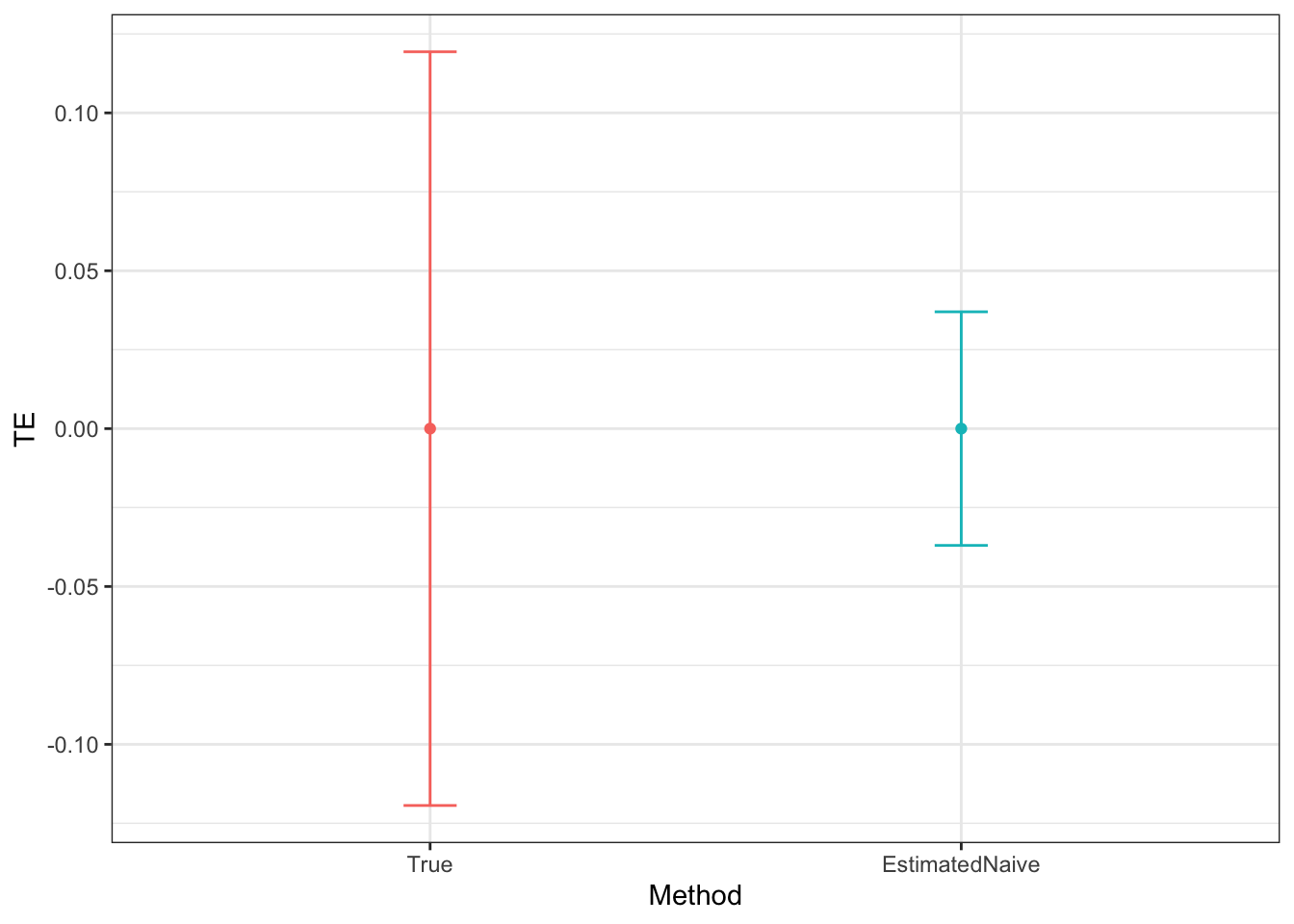
Figure 9.10: True vs estimated sampling noise under spatial autocorrelation
As we can see on the second plot on Figure 9.10, there is a major difference between the true and estimated sampling noise. Default OLS standard errors underestimate sampling noise severely: the true 99% level of sampling noise stemming from the Monte Carlo replications is equal to 0.18, while the sampling noise estimated using default OLS standard errors is equal to 0.1.
9.3.3 Estimating sampling noise with spatially autocorrelated data
Let us now study how to estimate sampling noise in data where there is spatial autocorrelation. There are at least three ways to do just that: either use the plug-in formula, estimate the covariance matrix of error terms \(\sigma^2\Omega\) and use Feasible Generalized Least Squares or use a covariance matrix robust to spatial correlation.
9.3.3.1 Using the plug-in formula
One possibility would be to use the plug-in formula in Theorem 9.3. It requires to determine \(k\), the number of neighbors (which is mostly a modelling choice, depending on the size of the pixel and on the shape of the contiguity matrix). Then one has to estimate \(\rho\), the correlation between the error term of unit \(i\) and of its neighbors. One quick way to do just that is to regress the estimated residuals \(\hat{U}_i\) on an average of the residuals of the neighbors of \(i\). Then, one has to estimate \(p\) and \(p_1\), which are simply the average proportion of treated units in the sample and among the neighbors of treated units, respectively.
This approach can be convenient as a quick fix but the formula is simplified by the existence of only one type of neighbors. In real life, influence might decrease over space more continuously. Also, this approach mostly works when the sample covers all space (like pixels, for example). In real life, samples might cover only part of the space, making \(k\) vary with each unit. A valid approach would be to use the average number of neighbors over the sample \(\bar{k}\) as an estimate of \(k\).
Example 9.9 Let’s see how this works in our example. The key is first to estimate the value of \(\rho\). \(\rho\) measures the correlation of the outcomes between two neighboring observations. One way to do just that is to estimate the average correlation between the error terms of all the units and of their neighbors. There are at least two ways to do that: sum all the products of the error terms of each individual and of its neighbors and divide by the total number of neighbors. Or sum all the products of the error terms for each unit with its neighbors, divide by the number of each unit’s neighbors, and then take the average of that. For the first approach, we can take the matrix of the products of the residuals, and multiply it by the matrix of neighbors, before it has been normalized by the number of neighbors at each line. The second approach uses the normalized matrix. Both approaches rely on taking the sum of the diagonal terms of the resulting product matrix, since this is where the terms corresponding to the neighbors of each unit are. Let’s go.
# Computing the matrix of the products of the residuals
UU <- U%*%t(U)
# First approach
Prod <- DistanceMatrixDiscrete20%*%UU
Rho.First <- sum(diag(Prod))/sum(rowSums(DistanceMatrixDiscrete20))
# Second approach
Prod.Second <- DistanceMatrixDiscreteWeights20%*%UU
Rho.Second <- sum(diag(Prod.Second))/nrow(DistanceMatrixDiscreteWeights20)
# mean number of neighbors
k <- mean(rowSums(DistanceMatrixDiscrete20))
Both approaches give consistent results: approach one gives \(\hat\rho=\) 0.01 and approach two gives \(\hat\rho=\) 0.02. Now, we need to compute \(k\). We use the mean number of neighbors: \(\hat k=\) 109. Finally, we need to compute \(p_1\), the average number of treated neighbors of treated units. For that, we can do the same thing as for estimating \(\rho\), except that we use the treatment indicator in the place of \(U\), and we use the second approach.
DD <- SpatialData$Ds%*%t(SpatialData$Ds)
ProdDD <- DistanceMatrixDiscreteWeights20%*%DD
p1 <- sum(diag(ProdDD))/sum(SpatialData$Ds)
p <- sum(SpatialData$Ds)/nrow(DistanceMatrixDiscreteWeights20)
CorrP1 <- (p1-p)/(p*(1-p))
Our estimates yield that \(\hat{p}_1=\) 0.57 and \(\hat{p}=\) 0.45. Let us now compute the correction term and our estimate of the variance of the with/without estimator:
Correction <- k*Rho.Second*CorrP1
VarWWSpatial <- (var(as.numeric(U))/(p*(1-p))*(1+Correction))/nrow(DistanceMatrixDiscreteWeights20)
SeWWPlugIn <- sqrt(VarWWSpatial)
Using the plug-in estimator, we estimate the standard error of the WW estimator to be equal to 0.02. Remember that the true standard error estimated over Monte Carlo replications is equal to 0.06 and that the naive standard error is: 0.02.
Remark. Extending this approach so that it is robust to heteroskedasticity is left as an exercise.
9.3.3.2 Using Feasible Generalized Least Squares
Another approach is to use Feasible Generalized Least Squares, by building an estimator \(\hat{\Omega}\) of the matrix \(\Omega\) is Assumption 9.3. We can then use the FGLS estimator \(\hatvar{\hat{\Theta}_{FGLS}}=(X'\hat{\Omega}_{FGLS}^{-1}X)^{-1}\).
Example 9.10 Let’s see how this works in our example.
In the previous section, we have computed an estimator of \(\rho\) and an estimator of \(\sigma^2\). We also know the structure of the matrix of neighbors. We can thus compute \(\hat{\Omega}\). Let’s go.
OmegaNeighbors <- Rho.Second*DistanceMatrixDiscrete20
OmegaSpatial <- var(as.numeric(U))*(Diagonal(nrow(DistanceMatrixDiscrete20),x=1)+Rho.Second*DistanceMatrixDiscrete20)
X <- matrix(c(rep(1,nrow(DistanceMatrixDiscrete20)),SpatialData$Ds),nrow=nrow(DistanceMatrixDiscrete20),ncol=2)
Var.Theta.FGLS <- solve(t(X)%*%solve(OmegaSpatial)%*%X)
SeWWFGLS <- sqrt(diag(Var.Theta.FGLS))[[2]]
Using the FGLS estimator, we estimate the standard error of the WW estimator to be equal to 0.02. Remember that the true standard error estimated over Monte Carlo replications is equal to 0.06 and that the naive standard error is: 0.02.
Remark. Extending this approach so that it is robust to heteroskedasticity is left as an exercise.
9.3.3.3 Using Spatial-Robust inference
Finally, the most widespread way to account for spatial autocorrelation is to use Conley (1999)’s standard errors. Conley proposes a way to estimate the covariance matrix of the parameters that is robust to (some degree of) spatial autocorrelation in the data. The original paper by Conley (1999) describes the proposed matrix in its equation (3.13), which is rather difficult to decipher. Fortunately, Conley (2016)’s Palgrave entry is less cryptic. Here, he writes his proposed estimator for the asymptotic distribution of the IV estimator in simpler terms. By analogy, and using the fact that OLS is simply that IV estimator using the explanatory variables as instruments for themselves, we can write Conley’s spatially-robust estimator as follows;
\[\begin{align*} \sqrt{N}(\hat{\Theta}_{OLS}-\Theta) & \sim \mathcal{N}\left(0,\left(\frac{1}{N}\sum_{i=1}^Nx_ix^{'}_i\right)^{-1}\hat{V}_N\left(\frac{1}{N}\sum_{i=1}^Nx_ix^{'}_i\right)^{-1'}\right) \\ \hat{V}_N & = \frac{1}{N}\sum_{i=1}^N\sum_{j=1}^NK_N(s_i,s_j)x_i\hat{\epsilon}_i(x_j\hat{\epsilon}_j)^{'}, \end{align*}\]
where \(x_i\) is the column vector of covariates for observation \(i\), \(\hat{\epsilon}_i\) is the estimated OLS residual, \(s_i\) are the spatial coordinates of observation \(i\) (for example its longitude and latitude) and \(K_N\) is a kernel function attributing weights to observation \(j\) as a function of its distance to observation \(i\). The most commonly used of such kernels is the uniform kernel, which takes value one when the distance between \(i\) and \(j\) is below some threshold and zero otherwise. This is the kernel we have used when building the \(W\) matrix in our example above (except that we have set the distance to zero when \(j=i\), and it is equal to \(1\) with the uniform kernel).
One thing that would be great is if we could write Conley’s estimator of the variance/covariance matrix in a fully matrix-style formula (without sums, but only using matrix products). One assumption that I entertain is that Conley’s matrix is actually identical to Leung (2020)’s matrix, with the entries in \(\mathcal{G}\) defined by the values of \(K_N(s_i,s_j)\). Let’s try to prove that. First, \(\sum_{i=1}^Nx_ix^{'}_i=X'X\), by the definition of the matrix product. Second, \(\sum_{i=1}^N\sum_{j=1}^NK_N(s_i,s_j)x_i\hat{\epsilon}_i(x_j\hat{\epsilon}_j)^{'}=\hat{\mathcal{M}}'G\hat{\mathcal{M}}\). This is because \(\hat{\mathcal{M}}'G=\left(\dots,\sum_{j=1}^NK_N(s_i,s_j)(x_j\hat{\epsilon}_j),\dots\right)\), and \(\hat{\mathcal{M}}'G\hat{\mathcal{M}}=\sum_{i=1}^Nx_i\hat{\epsilon}_i\sum_{j=1}^NK_N(s_i,s_j)(x_j^{'}\hat{\epsilon}_j)^{'}\), again by virtue of matrix multiplication. Finally, note that the terms in \((\frac{1}{N})^{-1}\) simplify, one with the \(\frac{1}{N}\) in \(\hat{V}_N\) and the other with the \(\frac{1}{N}\) stemming from the normalizing factor in \(\sqrt{N}(\hat{\Theta}_{OLS}-\Theta)\). Ok, so we have that Conley (1999)’s standard errors are a particular case of Leung (2020)’s matrix.
Example 9.11 Let’s see how this all works in our example.
Let us first start with Leung’s formula, and we will then move to the wonderful fixest package, which proposes a vcov_conley() function, but also has a vcov="conley" option.
# Let us first generate the G matrix, which is simply the DistanceMatrixDiscrete matrix plus a diagonal matrix of ones.
G.Conley <- DistanceMatrixDiscrete20+Diagonal(n=nrow(DistanceMatrixDiscrete20))
# Let us now generate the M and X matrices
# M has two columns: one for U*constant (vector of ones) and the other for U*Ds
# normally, the epsilons are used instead of the Us, with epsilon the residuals from an ols regression of U (or Y) on a constant and Ds
SpatialData <- SpatialData %>% mutate(UDs = U*Ds, Cst = 1)
M <- as.matrix(cbind(SpatialData$U,SpatialData$UDs))
X <- as.matrix(cbind(SpatialData$Cst,SpatialData$Ds))
# LEt us now compute Leung's matrix
VcovLeung <- ((solve(t(X)%*%X))%*%t(M)%*%G.Conley%*%M%*%(solve(t(X)%*%X)))
# SEWWConley
SEWWConley <- sqrt(diag(VcovLeung))[[2]]
Using Conley standard errors as implemented using Leung’s matrix, we estimate the standard error of the WW estimator to be equal to 0.05. Remember that the true standard error estimated over Monte Carlo replications is equal to 0.06 and that the naive standard error is: 0.02.
Let us now check what happens when we use the conley option in fixest.
# computing regression
RegSpatial <- feols(U~Ds,data=SpatialData)
VcovConleyFixest <- vcov_conley(RegSpatial,lat="latitude",lon="longitude",cutoff=20)
# SEWWConleyFixest
SEWWConleyFixest <- sqrt(diag(VcovConleyFixest))[[2]]
Using the fixestimplementation of Conley’s standard errors, we estimate the standard error of the WW estimator to be equal to 0.05.
Remember that the true standard error estimated over Monte Carlo replications is equal to 0.06 and that the naive standard error is: 0.02.
9.3.3.4 Monte Carlo simulations
Let us check what works best using Monte Carlo simulations of our data generating process. Actually, we already performed these simulations when we generated the Monte Carlo simulations to show the problem of autocorrelation with default standard errors. Let’s now just see how the estimators perform:
# plot
ggplot(Data.precision.Spatial,aes(x=Method,y=TE,color=Method,group=Method)) +
  geom_point() +
  geom_errorbar(aes(ymin=TE-1.96*Se,ymax=TE+1.96*Se,color=Method,group=Method),width=0.1)+
  theme_bw() +
theme(legend.position="none") 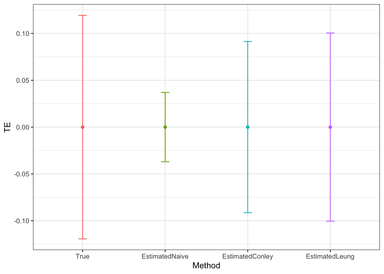
Figure 9.11: Estimated sampling noise under spatial autocorrelation
It seems that both Conley and Leung standard errors perform very well.
It is unclear why there are not eactly equivalent though, but it might be due to the treatment of degrees of freedom, or specifics in the way Conley standard errors are implemented in fixest.
Remark. One last question is how to choose the bandwidth of the social influence matrix.
Also, change social influence matrix of other methods to 20k to see if they work better then
9.4 Clustering on a network
A lot of datasets have a network flavor. A network is simply a set of observations with their accompanying links. A friendship network is the list of people and the list of their connections (who is friends with whom). In the case of a directed network (we also talk about directed graph), connections are unidirectionnal (I can be friends with you without you being friends with me). In an undirected network, connections are bidirectionnal (if I’m friends with you, you are friends with me). A network can also be a network of firms or countries that are trading with each other. A network can also be simply linked to geographic distance, or belonging to the same clusters (a firm or a village, for example). We are going to focus in undirected networks, because, for the purposes of autocorrelation and estimating standard errors, the nature of the network does not matter, all networks are considered undirected.
A key problem that might happen when you assign a treatment on a network is that the probability of receiving the treatment on some parts of the network is higher than in some others. If error terms are correlated among neighbors in the network, then we again have a problem that is akin to clustering. Since the units in the network are not i.i.d., we have less free variation than we think and thus the basic CLT fails. Something similar to the design effect is going to emerge, with the design effect increasing in the amount of auto-correlation in outcomes and in treatment.
Amazingly, the same solution as for clustering and spatial correlation works here. The Leung (2020) estimator for the covariance matrix of the parameters, which I have already partially introduced above in the context of clustering and spatial autocorrelation, is also going to be valid for estimating sampling noise on a network. In that case, the \(G\) matrix is such that \(G_{i,j}=1\) when \(i=j\), or when \(i\) and \(j\) are neighbors or when \(i\) and \(j\) share a neighbor, and zero otherwise. I am not going to study this approach in further detail since I will dedicate a whole chapter to Leung’s estimator when we study diffusion effects in Chapter 11.
9.5 Multi-way clustering
What if we go back to panel data, allow for temporal autocorrelation, but also accept that there will be some degree of cross-sectional autocorrelation, like clusters of observations who receive the same level of treatment? This would happen for example when treatment is clustered at a village, county or state level, for example, and the outcomes are also clustered in that way, while also being autocorrelated over time. Wages, for example, or employment, but also consumption, are outcomes that are autocorrelated both over space and over time. If we study the impact of minimum wage laws by using changes at the state-level in these laws, then we have exactly this problem, as has been argued by Bertrand et al. (2004) and Barrios et al. (2012). We are going to explore a few aspects of this issue in what follows, starting with the level at which we should cluster, the type of traditional estimators we can use and a finally a novel approach based on randomization inference.
9.5.1 At which level should we cluster?
A first key question is the level at which we should cluster our standard errors. It all sounds pretty arbitrary. And in a sense it still is, except in some cases, and we are going to see why and try to find ways to solve this issue.
9.5.1.1 Appropriate level of clustering in Randomized Controlled Trials
A first way to think about the issue of clustering is in the simplified environment of Randomized Controlled Trials. Barrios et al. (2012) shows that, under some not so restrictive assumptions, the proper level at which to account for clustering is the level at which the treatment is randomly assigned (or as good as randomly assigned). So if your treatment is randomized at the individual level, you do not need to cluster at all if you have cross sectional data, and you need to cluster at the individual level when you have panel data.
9.5.1.2 Appropriate level of clustering in natural experiments and observational methods
With natural experiments, things become murkier. Indeed, the treatment has not really been randomly assigned, but only as good as randomly (in the case of natural experiments) and not at all (or conditionnally on covariates) in observational methods. How the treatment is correlated spatially then matters and is not obvious. One way around this problem is to investigate spatial correlation in the treatment formally. One way to do just that, as suggested by Barrios et al. (2012), is to compute Mantel statistics for both treatment and outcomes (in first difference or as residuals of a regression ro reflect the estimation method). You should cluster at the maximum level where you detect autocorrelation for the treatment variable, or rather at the minimum between the maximum autocorrelation level of the outcome and the treatment. This approach is not applied in general in empirical research in economics, which therefore leaves a lot to the arbitrary judgement of authors and referees.
In panel data, in general, we tend to cluster at the state level for example, which means we also consider that all observations of the same state for different years are autocorrelated.
This is easy to implement with either the Leung approach (which is actually super adaptable: just use the contigguity matrix that makes sense for your application) or using fixest cluster option.
One tradition that seems to make sense is to try different levels of clustering and test the sensitivity of standard errors to those. Unfortunately, you then run into another problem: when the number of clusters gets small, CLT-based estimators (including block bootstrap) are biased and generally underestimate sampling noise. We will look at this issue in more detail in the next section.
Another approach is to leverage the exogenous source of variation and how it drives treatment allocation, and specifically at which spatial and temporal level. A cutting edge way of doing just that is to use Borusyak and Hull (2020)’s approach. Their approach is reserved for cases when one can express treatment exposure as a known combination of several influences, and only some of these influences are exogenous.
9.6 What to do when there are few clusters?
When the number of clusters becomes small (small is hard to define but anything below 42 seems small, and below 10 definitely is very small), the CLT-based approximations to the distribution of the treatment effect estimate are biased. This is because the residual variance is underestimated, as when sample size is small, because regression is overfitting and thus underestimating the residual variance. Simulations summarized in Tables VI and VIII of Bertrand et al. (2004) show that the rejection rate for a placebo law (so Type I error) moves from around the nominal 5% rate with 50 clusters, to 44% with 6 clusters for block bootstrap and to 11.5% with cluster robust standard errors, which is better but still more than double the nominal rate.
9.6.1 Aggregation
One extreme solution is to aggregate all the data at the cluster level, as suggested by Bertrand et al. (2004). With a treatment clustered at the state level, one could agrgegate outcomes in each state, for two periods: one before and one after the treatment. With a small number of covariates, one has to use a t-statistic correcting for the actual number of degrees of freedom, as suggested by Donald and Lang (2007). This approach works well in the simulations of Bertrand et al. (2004).
9.6.2 Permutation tests
Recently, Hagemann (2019) has proposed a randomization inference based approach to test for the existence of treatment effects with very few clusters (as low as 6, with 3 treated and 3 untreated). The test works as follows:
- Randomly select \(N_1\) clusters to be treated and \(N_0\) to be non treated among the existing clusters (where \(N_1\) and \(N_0\) are the actual numbers of treated and untreated clusters in your original sample).
- Estimate one regression per cluster and recover a critical parameter. For RCTs, the critical parameter is the intercept of the regression of the outcomes on the control variables. For DID, the critical parameter is the coefficient on the \(post\) dummy, that takes value one when the treatment is on, and zero otherwise.
- Compute the difference in means of the critical parameter in the treatment and control group.
- If \(N_1\neq N_0\), adjust this difference by a correction factor (a ratio of variance estimates)
- Compare the value of the resulting test statistic in the original sample to the distribution of the statistics with randomization inference, which is correct under the null. permutation (hagemann).
Remark. You can obtain confidence intervals using the usual method of computing test statistics for various values of the treatment effect.
Remark. Hagemann (2019) shows that this procedure is consistent (has correct size when the number of observations grows large), even if the number of clusters stays small. Hagemann (2023) proposes a similar test allowing for heteroskedasticity across clusters.
9.6.3 Wild bootstrap
Although the bootstrap does not work very well with a limited number of clusters, the wild cluster bootstrap seems to work better. As Cameron and Miller (2015) explain, the wild cluster bootstrap works as follows:
- Estimate the main model forcing the null assumption on the data. That is, for treatment effects models, run the regression without the main treatment indicator (the interaction between \(post\) and the treatment group in DID, for example).
- Recover the residuals \(\tilde{U}_{ic}\), with \(c\) the cluster index, and \(i\) the individual index.
- Randomly assign each cluster \(c\) a weight \(d_c=-1\) with probability \(0.5\) and \(d_c=1\) with probability \(0.5\).
- Generate new observations using your main model (either a constant in a simple RCT regression, or a constant, a time dummy and a treatment group dummy in a repeated cross section DID model, or a set of individual fixed effects and time fixed effects in a DID model in panel data) plus \(d_c\tilde{U}_{ic}\).
- Estimate the effect of the treatment using your preferred method on this new sample.
- Compare the original value of the treatment effect (or rather of the t-statistic) to its bootstrapped distribution (or rather to the bootstrapped distribution of the t-statistic).
Remark. This approach might have to be adapted somehow to work well with DID models à la Sun and Abraham. The extension is left as an exercise.
9.6.4 Ibragimov and Muller (2010) group-based inference
Ibragimov and Muller (2010) propose to estimate the parameter of interest in \(q\) groups that are approximately independent of each other, and to use the resulting distribution to build a test statistic on the mean of the parameter of interest, which will follow a \(t(q-1)\) distribution. For this approach to be consistent, you only need the size of each \(q\) group to increase to infinity, not \(q\) itself.
For DID applications, Ibragimov and Muller (2010) suggest to define the \(q\) groups as encompassing the level at which treatment varies (for example groups of contiguous states) and to compute the DID estimator for each group and then build the \(t\)-statistic for the null that the mean effect is zero. Confidence intervals will be valid.
For clustered RCTs, it all depends on whether (i) treatment is constant within clusters or not, (ii) we are willing to assume that each cluster is independent from its neighbors. If both assertions are true, then we can compute one treatment effect estimate in each cluster and then derive the distribution of the \(t\)-statistic.
For spatially clustered data, Ibragimov and Muller (2010) suggest to define groups as being block of observations located close to each other. With sufficiently large groups, inference will be based on mostly observations that are independent of each other.