Chapter 5 Observational Methods

In this lecture, we are going to study how to estimate the effect of an intervention on an outcome using observational methods, that is methods which try to correct for selection bias by accounting for as many observed confounders as possible. The key assumption that we are going to make is that of conditional independence:

Hypothesis 5.1 (Conditional Independence (in Expectation)) We assume that there exists a known set of observable covariates \(X_i\) such that:

\[\begin{align*} \esp{Y_i^0|X_i,D_i=1} & = \esp{Y_i^0|X_i,D_i=0}. \end{align*}\]

Under Assumption 5.1, the expected potential outcomes of the treated in the absence of the treatment are independent of the treatment conditional on a set of observed covariates \(X_i\). As a consequence, selection bias is zero after conditioning on \(X_i\), and we can recover the treatment on the treated parameter by using the With/Without comparison conditional on \(X_i\):

\[\begin{align*} \Delta^Y_{WW}(X_i) & = \esp{Y_i|X_i,D_i=1} - \esp{Y_i|X_i,D_i=0} \\ & = \esp{Y^1_i|X_i,D_i=1} - \esp{Y^0_i|X_i,D_i=0} \\ & = \esp{Y^1_i|X_i,D_i=1} - \esp{Y^0_i|X_i,D_i=1} \\ & = \esp{Y^1_i-Y_i^0|X_i,D_i=1}\\ & = \Delta^Y_{TT}(X_i), \end{align*}\]

where the third equality uses Assumption 5.1.

There are several ways to use Assumption 5.1 (and thus Assumption 5.2) to build estimators of the treatment effect. Let’s start with the parametric approaches and then we’ll study the non-parametric approaches.

Remark. Assumption 5.1 is the minimal assumption needed to indentify the average effect of the treatment on the treated. Researchers often use a stronger version of that assumption:

Hypothesis 5.2 (Conditional Independence) We assume that there exists a known set of observable covariates \(X_i\) such that:

\[\begin{align*} (Y_i^1,Y_i^0)\Ind D_i|X_i. \end{align*}\]

Assumption 5.2 is stronger than Assumption 5.1 because it imposes conditional independence of all the distribution of \(Y_i^0\), not only of its mean, and also because it imposes conditional independence of \(Y_i^1\) and moreover that this independence is jointly holding for \((Y_i^1,Y_i^0)\).

Remark. Assumptions 5.1 and 5.2 are sometimes called Ignorability, Unconfoundedness or Selection on Observables.

5.1 Parametric methods

We are going to study two approaches uses increasingly strong parametric assumptions. The first assumes the functional form of \(\esp{Y_i^0|X_i}\) is known. The second assumes furthermore that the functional form of \(\esp{Y_i^1|X_i}\) is known. We finaly are going to discuss the conditions under which a simple OLS regressions identifies the treatment effect on the treated.

5.1.1 Assuming \(\esp{Y_i^0|X_i}\) is known

Let’s study identification, estimation and inference when \(\esp{Y_i^0|X_i}\) is known

5.1.1.1 Identification

The most simple assumption that we can make in order to identify the treatment on the treated parameter under Conditional Indepedence is that the functional form of \(\esp{Y_i^0|X_i}\) is known (and for example is linear):

Hypothesis 5.3 We assume that there exists a known set of observable covariates \(X_i\) such that:

\[\begin{align*} \esp{Y_i^0|X_i} & = \alpha_0+\beta_0'X_i. \end{align*}\]

One way to use this assumption to identify the effect of the treatment on the treated is to follow the following steps:

Estimate \(\alpha_0\) and \(\beta_0\) on the population of untreated individuals.
Use these estimates to predict potential outcomes for the treated.
Compute the difference between the observed potential outcomes and the simulated ones for the treated observations.

In practice, this estimator, which I call \(\Delta^Y_{WWOLS(X)}\), is equal to:

\[\begin{align*} \Delta^Y_{WWOLS(X)} & = \esp{Y_i-\alpha_0-\beta_0'X_i|D_i=1}. \end{align*}\]

Under the assumptions we’ve made so far, \(\Delta^Y_{WWOLS(X)}\) identifies \(TT\):

Theorem 5.1 (Identification of TT using OLS) Under Assumptions 5.1 and (hyp:paramff0), TT is identified using the WW comparison adjusted by the OLS projection.

\[\begin{align*} \Delta^Y_{WWOLS(X)} & = \Delta^Y_{TT}. \end{align*}\]

Proof. Under Assumptions 5.1 and (hyp:paramff0), we have:

\[\begin{align*} \esp{Y_i^0|D_i=0,X_i} & = \esp{Y_i^0|X_i} = \alpha_0+\beta_0'X_i. \end{align*}\]

As a consequence, \(\alpha_0\) and \(\beta_0\) are identified by using the untreated population, as long as the components of \(X\) are not colinear. Then, we have:

\[\begin{align*} \Delta^Y_{WWOLS(X)} & = \esp{Y_i-\alpha_0-\beta_0'X_i|D_i=1}\\ & = \esp{Y_i-\esp{Y_i^0|D_i=1,X_i}|D_i=1}\\ & = \esp{Y_i|D_i=1}-\esp{\esp{Y_i^0|D_i=1,X_i}|D_i=1}\\ & = \esp{Y^1_i|D_i=1}-\esp{Y^0_i|D_i=1}\\ & = \Delta^Y_{TT}, \end{align*}\]

where the first equality is the definition of the second step of the OLS projection procedure, the second equality is a consequence of Assumptions 5.1 and (hyp:paramff0), the third and fifth equalities use the linearity of conditional expectations and the fourth equality uses the Law of Iterated Expectations.

5.1.1.2 Estimation

Estimation can follow in the sample steps similar to the ones taken in the population:

Estimate \(\hat{\alpha_0}\) and \(\hat{\beta_0}\) using an OLS regression of \(Y_i\) on \(X_i\) on the sample of untreated individuals.
Predict the counterfactual values for each treated using \(\hat{Y_i^0}=\hat{\alpha_0}+\hat{\beta_0}'X_i\).
Compute \(\hat{\Delta}^Y_{WWOLS(X)}=\frac{1}{\sum_{i=1}^ND_i}\sum_{i=1}^ND_i(Y_i^1-\hat{Y_i^0})\).

Example 5.1 Let’s see how this works in our example.

Let’s first choose some parameter values:

param <- c(8,.5,.28,1500,0.9,0.01,0.05,0.05,0.05,0.1)
names(param) <- c("barmu","sigma2mu","sigma2U","barY","rho","theta","sigma2epsilon","sigma2eta","delta","baralpha")

Let us now simulate the data:

\[\begin{align*} y_i^1 & = y_i^0+\bar{\alpha}+\theta\mu_i+\eta_i \\ y_i^0 & = \mu_i+\delta+U_i^0 \\ U_i^0 & = \rho U_i^B+\epsilon_i \\ y_i^B & =\mu_i+U_i^B \\ U_i^B & \sim\mathcal{N}(0,\sigma^2_{U}) \\ D_i & = \uns{y_i^B\leq\bar{y}} \\ (\eta_i,\mu_i,\epsilon_i) & \sim\mathcal{N}(0,0,0,\sigma^2_{\eta},\sigma^2_{\mu},\sigma^2_{\epsilon},0,0,0). \end{align*}\]

set.seed(1234)
N <-1000
mu <- rnorm(N,param["barmu"],sqrt(param["sigma2mu"]))
UB <- rnorm(N,0,sqrt(param["sigma2U"]))
yB <- mu + UB 
YB <- exp(yB)
Ds <- rep(0,N)
Ds[YB<=param["barY"]] <- 1 
epsilon <- rnorm(N,0,sqrt(param["sigma2epsilon"]))
eta<- rnorm(N,0,sqrt(param["sigma2eta"]))
U0 <- param["rho"]*UB + epsilon
y0 <- mu +  U0 + param["delta"]
alpha <- param["baralpha"]+  param["theta"]*mu + eta
y1 <- y0+alpha
Y0 <- exp(y0)
Y1 <- exp(y1)
y <- y1*Ds+y0*(1-Ds)
Y <- Y1*Ds+Y0*(1-Ds)

Let us now plot the sample and the procedure to estimate \(\hat{\Delta}^Y_{WWOLS(X)}\):

col.obs <- 'black'
col.unobs <- 'red'
lty.obs <- 1
lty.unobs <- 2
xlim.big <- c(-1.5,0.5)
xlim.small <- c(-0.15,0.55)
adj <- 0

# Sample

plot(yB[Ds==0],y0[Ds==0],pch=1,xlim=c(5,11),ylim=c(5,11),xlab="yB",ylab="Outcomes")
points(yB[Ds==1],y0[Ds==1],pch=1,col=col.unobs)
abline(v=log(param["barY"]),col=col.unobs)
legend(5,11,c('y0|D=0','y0|D=1'),pch=c(1,1),col=c(col.obs,col.unobs),ncol=1)

# Step 1
ols.reg.0 <- lm(y[Ds==0]~yB[Ds==0])

plot(yB[Ds==0],y0[Ds==0],pch=1,xlim=c(5,11),ylim=c(5,11),xlab="yB",ylab="Outcomes")
points(yB[Ds==1],y0[Ds==1],pch=1,col=col.unobs)
points(yB[Ds==0],ols.reg.0$fitted.values,col='blue')
abline(v=log(param["barY"]),col=col.unobs)
legend(5,11,c('y0|D=0','y0|D=1',expression(hat('y0|D=0'))),pch=c(1,1,1),col=c(col.obs,col.unobs,'blue'),ncol=2)

# step 2
y.pred <- ols.reg.0$coef[[1]]+ols.reg.0$coef[[2]]*yB[Ds==1]

plot(yB[Ds==0],y0[Ds==0],pch=1,xlim=c(5,11),ylim=c(5,11),xlab="yB",ylab="Outcomes")
points(yB[Ds==1],y0[Ds==1],pch=1,col=col.unobs)
points(yB[Ds==0],ols.reg.0$fitted.values,col='blue')
points(yB[Ds==1],y.pred,pch=3,col='blue')
abline(v=log(param["barY"]),col=col.unobs)
legend(5,11,c('y0|D=0','y0|D=1',expression(hat('y0|D=0')),expression(hat('y0|D=1'))),pch=c(1,1,1,3),col=c(col.obs,col.unobs,'blue','blue'),ncol=2)

# step 3
ww.ols <- mean(y[Ds==1]-y.pred)

plot(yB[Ds==0],y0[Ds==0],pch=1,xlim=c(5,11),ylim=c(5,11),xlab="yB",ylab="Outcomes")
points(yB[Ds==1],y0[Ds==1],pch=1,col=col.unobs)
points(yB[Ds==0],ols.reg.0$fitted.values,col='blue')
points(yB[Ds==1],y.pred,col='blue')
points(yB[Ds==1],y[Ds==1],pch=3,col='black')
abline(v=log(param["barY"]),col=col.unobs)
legend(5,11,c('y0|D=0','y0|D=1','y1|D=1',expression(hat('y0|D=0')),expression(hat('y0|D=1'))),pch=c(1,1,3,1,3),col=c(col.obs,col.unobs,col.obs,'blue','blue'),ncol=2)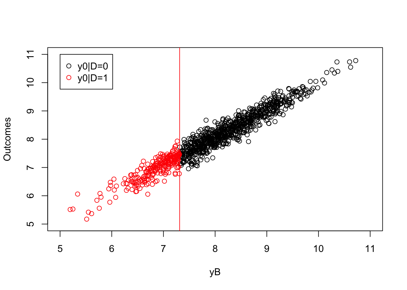

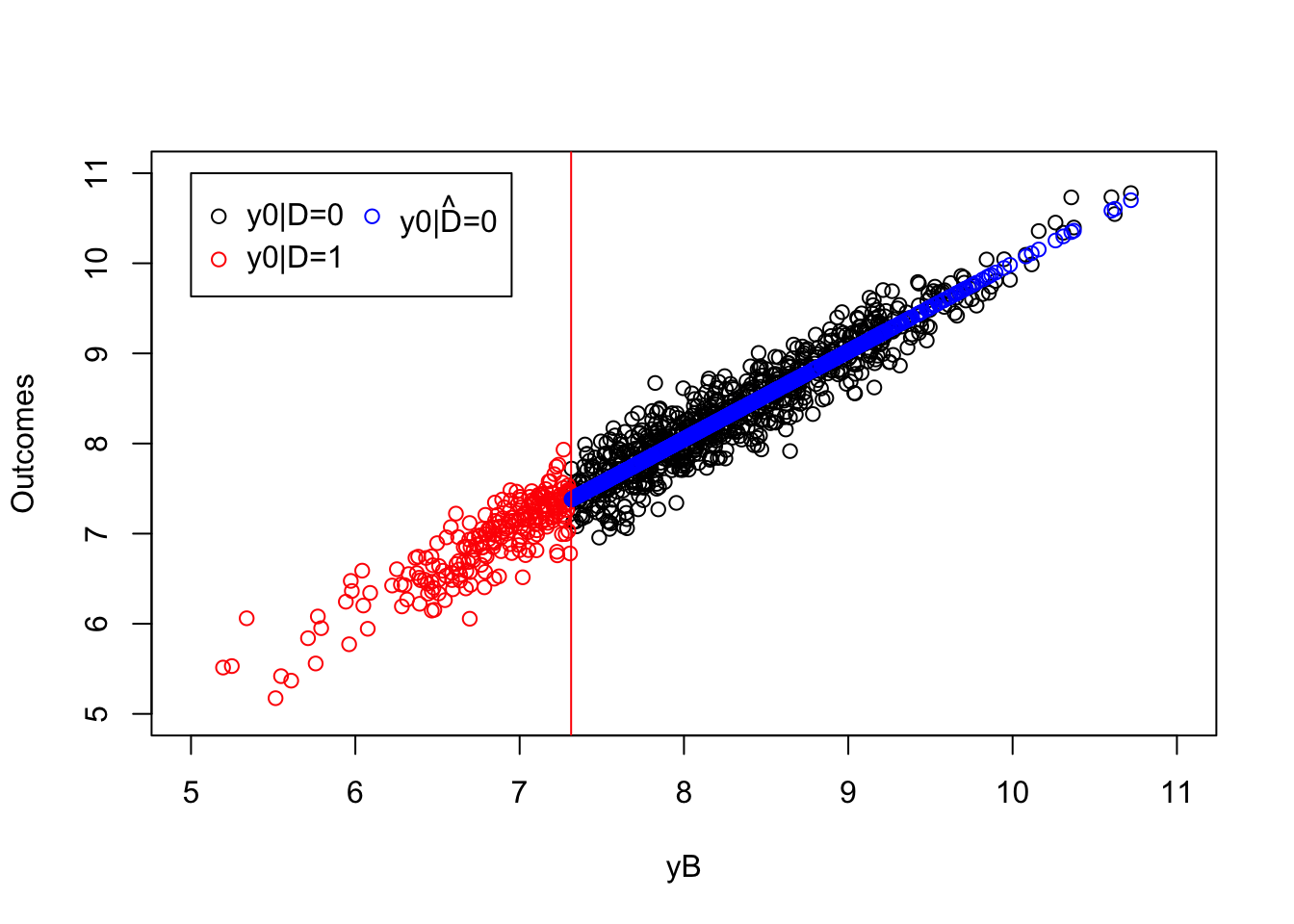
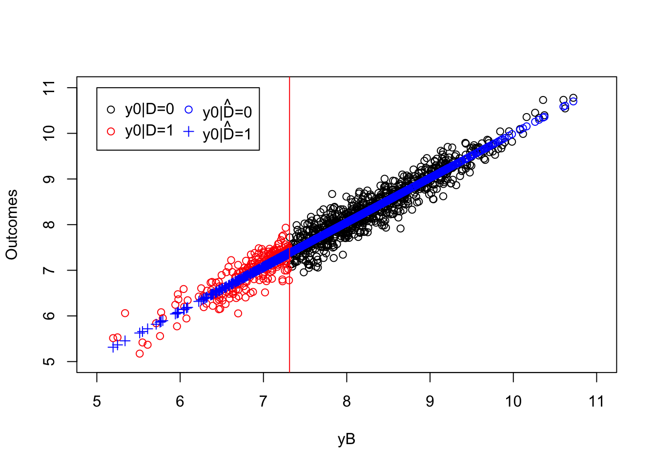
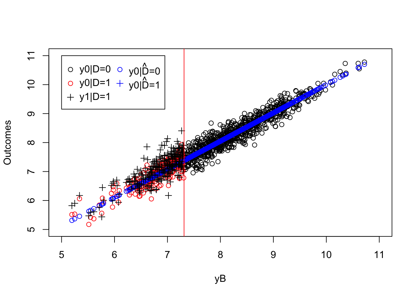
Estimating treatment effects using WWOLS(X)

Figure 5.1: Estimating treatment effects using WWOLS(X)

Let’s also compute the true values of the treatment effects in the population:

delta.y.tt <- function(param){
  return(param["baralpha"]+param["theta"]*param["barmu"]-param["theta"]*((param["sigma2mu"]*dnorm((log(param["barY"])-param["barmu"])/(sqrt(param["sigma2mu"]+param["sigma2U"]))))/(sqrt(param["sigma2mu"]+param["sigma2U"])*pnorm((log(param["barY"])-param["barmu"])/(sqrt(param["sigma2mu"]+param["sigma2U"]))))))
}

delta.y.ate <- function(param){
  return(param["baralpha"]+param["theta"]*param["barmu"])
}

The true effect of the treatment on the treated in the population is equal to 0.17 and our estimator, \(\hat{\Delta}^Y_{WWOLS(X)}\), is equal to 0.18.

5.1.1.3 Estimating precision

Estimating the precision of this estimator can be done using the bootstrap. Or we could derive its distribution using the CLT.

TO DO

5.1.2 Assuming \(\esp{Y_i^1|X_i}\) is known

One way to make our estimation procedure even simpler than using the \(WWOLS(X)\) estimator is to assume that \(\esp{Y_i^1|X_i}\) is also linear. In that case, we are going to be able to use the OLS estimator conditioning on \(X_i\) to estimate the average treatment effect on the treated. We are going to see that this estimator will have a peculiar shape. We’ll understand better why in Section 5.1.3. Let’s start with how to use OLS under linearity of conditional expectations.

5.1.2.1 Identification

Let’s assume that we also know the functional form of \(\esp{Y_i^1|X_i}\):

Hypothesis 5.4 We assume that there exists a known set of observable covariates \(X_i\) such that:

\[\begin{align*} \esp{Y_i^1|X_i} & = \alpha_1+\beta_1'X_i. \end{align*}\]

The first thing we can show is that we now have a parametric formula for our target parameter \(TT\) (using the slighlty stronger version of the Conditional Indepedence Assumption):

Theorem 5.2 (TT under Linearity of Conditional Expectations) Under Assumptions 5.2, 5.3 and 5.4, the Treatment on the Treated parameter simplifies to:

\[\begin{align*} \Delta^Y_{TT} & = \alpha_1-\alpha_0+(\beta_1-\beta_0)'\esp{X_i|D_i=1}. \end{align*}\]

Proof. \[\begin{align*} \Delta^Y_{TT} & = \esp{Y_i^1-Y_i^0|D_i=1} \\ & = \esp{\esp{Y_i^1-Y_i^0|X_i,D_i=1}|D_i=1} \\ & = \esp{\esp{Y_i^1|X_i,D_i=1}-\esp{Y_i^0|X_i,D_i=1}|D_i=1} \\ & = \esp{\esp{Y_i^1|X_i}-\esp{Y_i^0|X_i}|D_i=1} \\ & = \esp{\alpha_1+\beta_1'X_i-(\alpha_0+\beta_0'X_i)|D_i=1} \\ & = \alpha_1-\alpha_0+(\beta_1-\beta_0)'\esp{X_i|D_i=1}, \end{align*}\]

where the second equality follows from the Law of Iterated Exppectations, the third equality from Assumption 5.2 and the fourth equality from Assumptions 5.3 and 5.4.

Remark. Theorem 5.2 shows that under our assumptions, treatment effects are heterogenous in a way that is correlated with the treatment only because of differences in \(X_i\).

Equipped with this result, we can now state the identification result of this section:

Theorem 5.3 (OLS Identifies TT under Linearity and Conditional Independence) Under Assumptions 5.2, 5.3 and 5.4, the OLS coefficient \(\delta\) in the following regression:

\[\begin{align*} Y_i & = \alpha_0 + \beta_0'X_i + (\beta_1-\beta_0)'\left(X_i-\esp{X_i|D_i=1}\right)D_i + \delta D_i + U_i \end{align*}\]

identifies the effect of the treatment on the treated.

We denote: \(\delta=\Delta^Y_{OLS(X)}\).

Proof. Under Assumptions 5.3 and 5.4, we have \(Y_i^d=\alpha_d + \beta_d'X_i +Y_i^d-\esp{Y_i^d|X_i}\), for \(d\in\left\{0,1\right\}\). As a consequence, we have:

\[\begin{align*} Y_i & = Y_i^0+D_i(Y_i^1-Y_i^0) \\ & = \alpha_0 + \beta_0'X_i +D_i(\alpha_1-\alpha_0 + (\beta_1-\beta_0)'X_i)\\ & \phantom{=}+Y_i^0-\esp{Y_i^0|X_i}+D_i(Y_i^1-Y_i^0-(\esp{Y_i^1|X_i}-\esp{Y_i^0|X_i}))\\ & = \alpha_0 + \beta_0'X_i + (\beta_1-\beta_0)'\left(X_i-\esp{X_i|D_i=1}\right)D_i + (\alpha_1-\alpha_0 + (\beta_1-\beta_0)'\esp{X_i|D_i=1})D_i\\ & \phantom{=}+\underbrace{Y_i^0-\esp{Y_i^0|X_i}+D(Y_i^1-Y_i^0-\esp{Y_i^1-Y_i^0|X_i})}_{U_i}\\ & = \alpha_0 + \beta_0'X_i + (\beta_1-\beta_0)'\left(X_i-\esp{X_i|D_i=1}\right)D_i + \Delta^Y_{TT}D_i +U_i, \end{align*}\]

where the first equation uses the Switching Equation, the second equation uses Assumptions 5.3 and 5.4 and the last equation uses Theorem 5.2.

We are now going to show that \(\esp{U_i|X_i,D_i}=0\).

\[\begin{align*} \esp{U_i|X_i,D_i=0} & = \esp{Y_i^0-\esp{Y_i^0|X_i}|X_i,D_i=0}\\ & =\esp{Y_i^0|X_i,D_i=0}-\esp{\esp{Y_i^0|X_i}|X_i,D_i=0}\\ & =\esp{Y_i^0|X_i,D_i=0}-\esp{\esp{Y_i^0|X_i,D_i=0}|X_i,D_i=0}\\ & =\esp{Y_i^0|X_i,D_i=0}-\esp{Y_i^0|X_i,D_i=0}\\ & = 0\\ \esp{U_i|X_i,D_i=1} & = \esp{Y_i^0-\esp{Y_i^0|X_i}|X_i,D_i=1}+\esp{Y_i^1-Y_i^0-\esp{Y_i^1-Y_i^0|X_i}|X_i,D_i=1}\\ & =\esp{Y_i^1-Y_i^0|X_i,D_i=1}-\esp{\esp{Y_i^1-Y_i^0|X_i}|X_i,D_i=1} \\ & =\esp{Y_i^1-Y_i^0|X_i,D_i=1}-\esp{\esp{Y_i^1-Y_i^0|X_i,D_i=1}|X_i,D_i=1} \\ & = 0, \end{align*}\]

where the third and eighth equalities follow from Assumption 5.2.

We thus have \(\esp{Y_i|X_i,D_i}=\alpha_0 + \beta_0'X_i + (\beta_1-\beta_0)'\left(X_i-\esp{X_i|D_i=1}\right)D_i + \Delta^Y_{TT}D_i\). Theorem A.2 ensures that the OLS estimator identifies the parameters of this model. As a consequence, \(\Delta^Y_{TT}\) is identified by the OLS estimator of \(\delta\) in the model. This completes the proof.

5.1.2.2 Estimation

What is pretty nice with Theorem 5.3 is that it suggests directly an estimation strategy. Let’s estimate \(\hat\delta^{OLS}\) in the following regression:

\[\begin{align*} Y_i & = \alpha_0 + \beta_0'X_i + (\beta_1-\beta_0)'\left(X_i-\esp{X_i|D_i=1}\right)D_i + \delta D_i + U_i. \end{align*}\]

Example 5.2 Let’s see what happens in our example when doing that.

# deameaning the control variable
yB.Ds <-(yB-mean(yB[Ds==1]))*Ds
# running the OLS estimator with interactions between treatment and demeaned covariate
ols.direct <- lm(y~yB+Ds+yB.Ds)
# estimate of TT
ww.ols.direct <- ols.direct$coef[[3]]

Our estimator is equal to 0.18, while the true effect of the treatment on the treated in the population is equal to 0.17.

Monte Carlo simulations

5.1.2.3 Estimating precision

Estimating precision is pretty straightforward in our case. What is going to happen with respect to a simple WW estimator that does not condition on covariates is that the asymptotic variance of the estimated treatment effect is going to depend on the variance of outcomes conditional on observed covariates \(X_i\). As a consequence, and as we have already seen in Chapter 3, precision will increase as long as the covariates we control for explain part of the variance of the outcome. The main issue that we have to deal with is that of heteroskedasticity: \(U_i\) is correlated with both \(X_i\) and \(D_i\). So we need to use a heteroskedasticity-robust estimator for the variance of the treatment effect. Let us first state the main result. For that, we need to reformulate the classical assumptions so that they cover the case with covariates:

Hypothesis 5.5 (i.i.d. sampling with covariates) We assume that the observations in the sample are identically and independently distributed:

\[\begin{align*} \forall i,j\leq N\text{, }i\neq j\text{, } & (Y_i,D_i,X_i)\Ind(Y_j,D_j,X_j),\\ & (Y_i,D_i,X_i)\&(Y_j,D_j,X_j)\sim F_{Y,D,X}. \end{align*}\]

Hypothesis 5.6 (Finite variances of potential outcomes conditional on covariates) We assume that \(\var{Y_i^1|X_i,D_i=1}\) and \(\var{Y_i^0|X_i,D_i=0}\) are finite.

We can now state our main result:

Theorem 5.4 (Distribution of the OLS Estimator of TT under Conditional Independence) Under Assumptions 5.2, 5.3, 5.4, 2.1, 5.5 and 5.6, we have:

\[\begin{align*} \sqrt{N}(\hat\Delta^Y_{OLS(X)}-\Delta^Y_{TT}) & \stackrel{d}{\rightarrow} \mathcal{N}\left(0,\frac{\var{Y^0_i|X_i,D_i=0}}{1-p}+\frac{\var{Y^1_i|X_i,D_i=1}}{p}\right), \end{align*}\]

with \(p=\Pr(D_i=1)\).

Proof. See Section A.4.1 in the Appendix.

Remark. Theorem 5.4 is super powerful: it tells us that conditioning on observed covariates yields an improvement in precision equivalent to the part of the variance of \(Y_i\) explained by the observed covariates. What is nice as well is that the distribution of the OLS estimator with controls has the same flavor as the distribution of the silpler With/Without estimator derived in Theorem 2.5 (and in Lemma A.5).

Remark. In order to operationalize Theorem 5.4, one can either use the formula or simply use the heteroskedasticity-robust variance-covariance matrix proposed for the OLS estimator. Both estimators should be similar. Let \(\Theta=(\alpha_0,\beta_0,\beta_1,\delta)\) and \(X\) be the matrix of all regressors, with a first column of ones and the last column of \(D_i\). Most available heteroskedasticity robust estimators based on the CLT can be written in the following way:

\[\begin{align*} \var{\hat{\Theta}_{OLS}} & \approx (X'X)^{-1}X'\hat{\Omega}X(X'X)^{-1}, \end{align*}\]

where \(\hat{\Omega}=\diag(\hat{\sigma}^2_{U_1},\dots,\hat{\sigma}^2_{U_N})\) is an estimate the covariance matrix of the residuals \(U_i\).

Here are various classical estimators for \(\hat{\Omega}\):

\[\begin{align*} \text{HC0:} & & \hat{\sigma_{U_i}}^2 & = \hat{U_i}^2 \\ \text{HC1:} & & \hat{\sigma_{U_i}}^2 & = \frac{N}{N-K}\hat{U_i}^2 \\ \text{HC2:} & & \hat{\sigma_{U_i}}^2 & = \frac{\hat{U_i}^2}{1-h_i} \\ \text{HC3:} & & \hat{\sigma_{U_i}}^2 & = \frac{\hat{U_i}^2}{(1-h_i)^2}, \end{align*}\]

where \(\hat{U}_i\) is the residual from the OLS regression, \(K\) is the number of regressors, \(h_i\) is the leverage of observation \(i\), and is the \(i^{\text{th}}\) diagonal element of \(H=X(X'X)^{-1}X'\). HC1 is the one reported by Stata when using the ‘robust’ option. All of these estimators are programmed in the sandwich package.

Example 5.3 Let’s see how our estimator works to estimate precision.

We can first try to implement the formula.

# regs on X in both smaples
ols.reg.0 <- lm(y[Ds==0]~yB[Ds==0])
ols.reg.1 <- lm(y[Ds==1]~yB[Ds==1])

# variance
var.delta.ols <- 1/N*(var(ols.reg.0$residuals)/(1-mean(Ds))+var(ols.reg.1$residuals)/(mean(Ds)))

We can now try to see what the heteroskedasticity-robust variance estimator gives.

ols.direct.HC1 <- vcovHC(ols.direct,type='HC1')

The robust standard error using HC1 is thus 0.03, while the default standard error assuming homoskedasticity is 0.03. The estimate obtained using Theorem 5.4 directly is equal to 0.02.

5.1.3 Properties of the OLS estimator under Conditional Independence

As we have seen in Chapter 3, we could also have estimated \(TT\) using a regression omitting the interaction between the treatment indicator and control variables. With RCTs, this did not matter for the final result. With Observational Methods, this might make a huge difference. The reason is that the distribution of the observed covariates in the treatment and control group are the same in expectation in an RCT, while they are by essence different under Conditional Independence. As a consequence, when we estimate a model by OLS which does not insert interactions of the covariates, we might end up with a different parameter than the one we are after.

Sloczynski (2020) studies this issue in great detail (Goldsmith-Pinkham, Hull and Kolesar (2022) make also progress on this front, but in a more general way.) In order to derive his result, Sloczynski (2020) slightly strengthens the assumptions we have made so far, especially by making potential outcomes dependent on \(X_i\) only through the propensity score: \(p(X_i)=\Pr(D_i=1|X_i)\). Sloczynski (2020)’s main result concerns \(\delta\) estimated by OLS in the following regression:

\[\begin{align*} Y_i & = \alpha + \beta' X_i + \delta D_i + U_i. \end{align*}\]

Theorem 5.5 (Weighted Average Interpretation of OLS) Under Assumptions 5.1, 5.3, 5.4, 5.6 (modified to hold with \(p(X_i)\) replacing \(X_i\)) and assuming that \(\esp{Y_i^2}\) and \(\esp{\lVert X_i^2 \rVert}\) are finite and that the covariance matrix of \((D_i,X_i)\) is non singular, we have \(\delta\) in the previous equation when estimated by OLS equal to:

\[\begin{align*} \delta^{OLS} & = w_1\Delta^Y_{TT}+w_0\Delta^Y_{TUT}, \end{align*}\]

with:

\[\begin{align*} w_1 & = \frac{(1-p)\var{p(X_i)|D_i=0}}{p\var{p(X_i)|D_i=1}+(1-p)\var{p(X_i)|D_i=0}}\\ w_0 & = \frac{p\var{p(X_i)|D_i=1}}{p\var{p(X_i)|D_i=1}+(1-p)\var{p(X_i)|D_i=0}} = 1-w_1. \end{align*}\]

and \(p=\Pr(D_i=1)\).

Proof. See Sloczynski (2020).

Remark. Theorem 5.5 shows that OLS without interactions between the treatment and the covariates is a weighted average of the effect of the treatment on the treated (\(\Delta^Y_{TT}\)) and of the effect of the treatment on the untreated (\(\Delta^Y_{TUT}=\esp{Y_i^1-Y_i^0|D_i=1}\)). This is thus not the parameter we are after. Fortunately, the weights are positive and sum to one, so that we still find a weighted average of treatment effects with positive weights Unfortunately, the weigths do not behave as we would like. For example, \(w_1\), the weight on \(TT\), becomes larger as the proportion of the UNtreated increases. This is inconvenient for estimating the \(ATE\). It is also inco,venient for estimating \(TT\), since how close \(\delta^{OLS}\) is to \(TT\) depends on whether there are a lot of treated units in the population (in which case \(\delta^{OLS}\) will be closer to \(TUT\)) or not (in which case, \(\delta^{OLS}\) will be closer to \(TT\)).

Example 5.4 Let’s see how this result plays out in our example. Note however than treatment effect heterogeneity might not be enough to alter our estimates strongly.

Let’s estimate a model without interactions:

# running the OLS estimator without interactions
ols.simp <- lm(y~yB+Ds)
# estimate of TT
ww.ols.simp <- ols.simp$coef[[3]]

The estimate of \(TT\) using the OLS regression without interactions is equal to 0.182, while our estimate obtained with the added interaction term is equal to 0.184.

5.1.4 Problems with parametric methods

When the conditional expectation of outcomes given the covariates is not linear, parametric methods which make this assumption will be erroneous. We will talk of specification bias.

Example 5.5 Let’s see why in our example:

We write outcomes as a non linear function of the pre-treatment covariate \(y_i^B\):

\[\begin{align*} y^0_i & =\mu_i+\delta+\gamma (y_i^B - \bar{y^B})^2 + U_i^0. \end{align*}\]

Let’s choose some parameters:

param <- c(param,0.1,7.98)
names(param) <- c("barmu","sigma2mu","sigma2U","barY","rho","theta","sigma2epsilon","sigma2eta","delta","baralpha","gamma","baryB")

and then simulate a dataset:

set.seed(1234)
N <-1000
mu <- rnorm(N,param["barmu"],sqrt(param["sigma2mu"]))
UB <- rnorm(N,0,sqrt(param["sigma2U"]))
yB <- mu + UB 
YB <- exp(yB)
Ds <- rep(0,N)
Ds[YB<=param["barY"]] <- 1 
epsilon <- rnorm(N,0,sqrt(param["sigma2epsilon"]))
eta<- rnorm(N,0,sqrt(param["sigma2eta"]))
U0 <- param["rho"]*UB + epsilon
y0 <- mu +  U0 + param["delta"] + param["gamma"]*(yB-param["baryB"])^2
alpha <- param["baralpha"]+  param["theta"]*mu + eta
y1 <- y0+alpha
Y0 <- exp(y0)
Y1 <- exp(y1)
y <- y1*Ds+y0*(1-Ds)
Y <- Y1*Ds+Y0*(1-Ds)

If we estimate the conditional expectation on the untreated population using a linear model, we are going to have biased predictions of the truth. Let’s first estimate the regression function:

ols.reg.0 <- lm(y[Ds==0]~yB[Ds==0])
# predicted values for the treated
y.pred <- ols.reg.0$coef[[1]]+ols.reg.0$coef[[2]]*yB[Ds==1]
# estimated treatment effect by WWOLSX
ww.ols <- mean(y[Ds==1]-y.pred)
# true value of TT in the sample
tt.sample <- mean(alpha[Ds==1])

plot(yB[Ds==0],y0[Ds==0],pch=1,xlim=c(5,11),ylim=c(5,11),xlab="yB",ylab="Outcomes")
points(yB[Ds==1],y0[Ds==1],pch=1,col='red')
points(yB[Ds==0],ols.reg.0$fitted.values,col='blue')
points(yB[Ds==1],y.pred,pch=3,col='blue')
points(yB[Ds==1],y[Ds==1],pch=3,col='black')
abline(v=log(param["barY"]),col='red')
legend(5,11,c('y0|D=0','y0|D=1','y1|D=1',expression(hat('y0|D=0')),expression(hat('y0|D=1'))),pch=c(1,1,3,1,3),col=c('black','red','black','blue','blue'),ncol=2)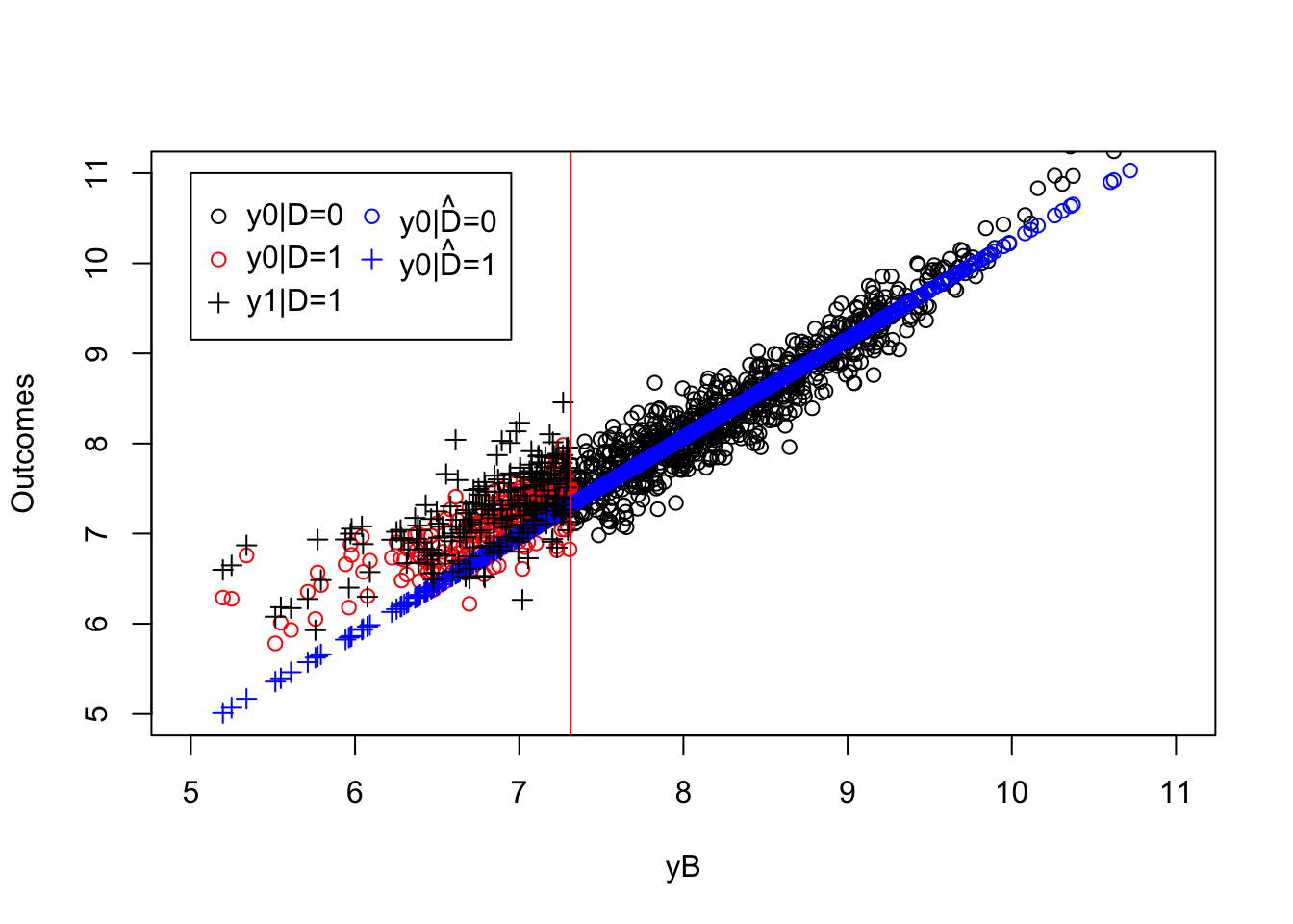

Figure 5.2: Biased parametric estimator

We can see on Figure 5.2 that the predicted values for the potential outcomes of the treated in the absence of the treatment (\(\hatesp{y_i^0|D_i=1,y_i^B}\)) based on the regression estimated on the untreated observations (in blue) are too low compared with the true values (in red). As a consequence, the OLS estimator is going to over estimate the true effect of the treatment. Indeed, the OLS estimate of the effect of the treatment is equal to 0.45 while the true value of the treatment effect in the sample is equal to 0.16.

5.2 Nonparametric methods

Nonparametric observational methods enable to avoid (or at least mitigate) the issue of specification bias. In exchange, they have stronger requirements than parametric methods in terms of comparability between treated and control observations. The idea is that nonparametric methods rely on local comparisons to avoid specification bias. For that, we need that treated and untreated observations overlap. We call this assumption the Common Support Assumption, and it is required for nonparametric methods to solve the issue of specification bias.

Hypothesis 5.7 (Common Support) We assume that, for the known set of observable covariates \(X_i\) for which the Selection on Observables Assumption holds, we have:

\[\begin{align*} 0<\Pr(D_i=1|X_i)<1. \end{align*}\]

Example 5.6 Assumption 5.7 does not hold on Figure 5.2. The probability of receiving treatment jumps discontinuously at \(y_i^B=\bar{y}\) from \(1\) to \(0\).

Let’s generate some data with common support. For that, we are going to modify the selection equation to add some noise so that units with similar \(y_i^B\) might end up treated or untreated:

\[\begin{align*} D_i & = \uns{y_i^B+V_i\leq\bar{y}} \\ V_i & \Ind Y_i^0 \\ V_i & \sim\mathcal{N}(0,\sigma^2_{\mu}+\sigma^2_{U}) \end{align*}\]

Let’s now generate some data following this new selection equation:

set.seed(1234)
mu <- rnorm(N,param["barmu"],sqrt(param["sigma2mu"]))
UB <- rnorm(N,0,sqrt(param["sigma2U"]))
yB <- mu + UB 
YB <- exp(yB)
Ds <- rep(0,N)
V <- rnorm(N,0,sqrt(param["sigma2mu"]+param["sigma2U"]))
Ds[yB+V<=log(param["barY"])] <- 1 
epsilon <- rnorm(N,0,sqrt(param["sigma2epsilon"]))
eta<- rnorm(N,0,sqrt(param["sigma2eta"]))
U0 <- param["rho"]*UB + epsilon
y0 <- mu +  U0 + param["delta"] + param["gamma"]*(yB-param["baryB"])^2
alpha <- param["baralpha"]+  param["theta"]*mu + eta
y1 <- y0+alpha
Y0 <- exp(y0)
Y1 <- exp(y1)
y <- y1*Ds+y0*(1-Ds)
Y <- Y1*Ds+Y0*(1-Ds)

Let’s plot this new dataset and examine it for common support:

par(mar=c(5,4,4,5))
plot(yB[Ds==0],y0[Ds==0],pch=1,xlim=c(5,11),ylim=c(5,11),xlab="yB",ylab="Outcomes")
points(yB[Ds==1],y[Ds==1],pch=3,col='blue')
abline(v=log(param["barY"]),col='red')
legend(5,10.5,c('y0|D=0','y1|D=1','D'),pch=c(1,3,2),col=c(col.obs,'blue',col.unobs),ncol=1)
par(new=TRUE)
plot(yB,Ds,pch=2,col=col.unobs,xlim=c(5,11),xaxt="n",yaxt="n",xlab="",ylab="")
axis(4)
mtext("D",side=4,line=3)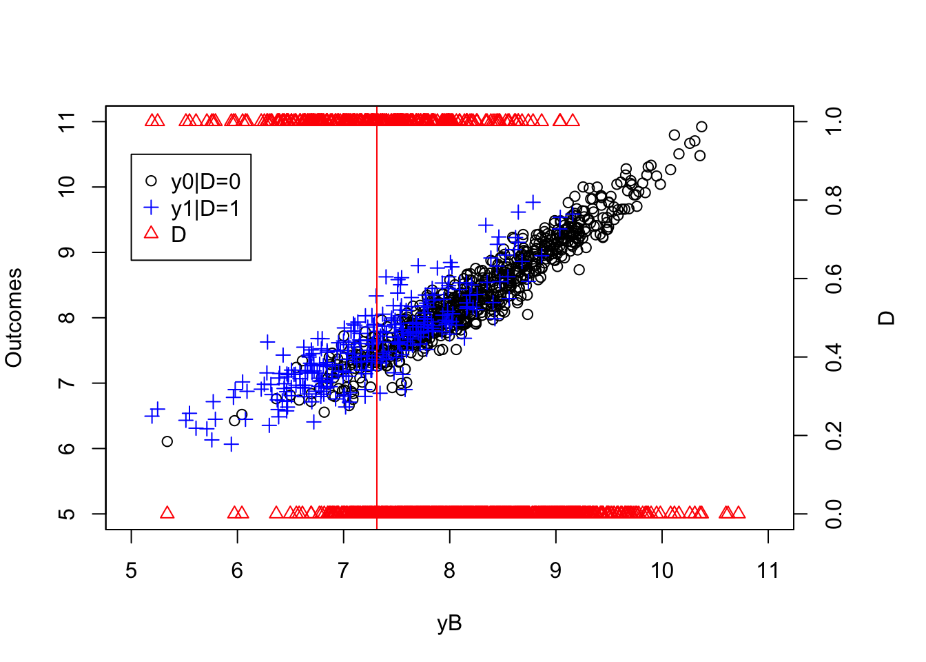

Figure 5.3: Common Support Holds

Figure 5.3 shows that we now have treated and untreated units on both sides of \(y_i^B=\bar{y}\). Before we move to the identification of \(TT\) under Assumption 5.7, we need to compute the true value of the \(TT\) parameter in the population in our new example: Because we have changed the selection rule, the value of \(TT\) in the population has changed also:

\[\begin{align*} \Delta_{TT}^y & =\bar{\alpha}+\theta\bar{\mu} -\theta\frac{\sigma^2_{\mu}}{\sqrt{2(\sigma^2_{\mu}+\sigma^2_{U})}}\frac{\phi\left(\frac{\bar{y}-\bar{\mu}}{\sqrt{2(\sigma^2_{\mu}+\sigma^2_{U})}}\right)}{\Phi\left(\frac{\bar{y}-\bar{\mu}}{\sqrt{2(\sigma^2_{\mu}+\sigma^2_{U})}}\right)}. \end{align*}\]

Let’s write a fiunction to compute this parameter:

delta.y.tt.com.supp <- function(param){
  return(param["baralpha"]+param["theta"]*param["barmu"]-param["theta"]*((param["sigma2mu"]*dnorm((log(param["barY"])-param["barmu"])/(sqrt(2*(param["sigma2mu"]+param["sigma2U"])))))/(sqrt(2*(param["sigma2mu"]+param["sigma2U"]))*pnorm((log(param["barY"])-param["barmu"])/(sqrt(2*(param["sigma2mu"]+param["sigma2U"])))))))
}
delta.y.tt.CS.pop <- delta.y.tt.com.supp(param)

The value of \(TT\) in the population in our new example is 0.18.

5.2.1 Identification

Let’s now derive identification of \(TT\):

Theorem 5.6 (Identification of TT Under Conditional Independence and Common Support) Under Assumptions 5.1 (or the stronger 5.2) and 5.7, \(TT\) is identified using either a nonparametric regression approach or a reweighting approach:

\[\begin{align*} \Delta^Y_{TT} & = \Delta^Y_{NPR(X)} = \Delta^Y_{RW(X)}, \end{align*}\]

with:

\[\begin{align*} \Delta^Y_{NPR(X)} & = \esp{Y_i-\esp{Y_i|X_i,D_i=0}|D_i=1} \\ \Delta^Y_{RW(X)} & = \esp{Y_i|D_i=1} \\ & \phantom{=} -\esp{Y_i\frac{\Pr(D_i=1|X_i)}{1-\Pr(D_i=1|X_i)}\frac{1-\Pr(D_i=1)}{\Pr(D_i=1)}|D_i=0}. \end{align*}\]

Proof. Let us start with the first equality:

\[\begin{align*} \Delta^Y_{NPR(X)} & = \esp{Y_i-\esp{Y_i|X_i,D_i=0}|D_i=1} \\ & = \esp{Y_i|D_i=1}-\esp{\esp{Y_i|X_i,D_i=0}|D_i=1}\\ & = \esp{Y^1_i|D_i=1}- \esp{\esp{Y^0_i|X_i,D_i=0}|D_i=1} \\ & = \esp{Y^1_i|D_i=1}- \esp{\esp{Y^0_i|X_i,D_i=1}|D_i=1} \\ & = \esp{Y^1_i|D_i=1}- \esp{Y^0_i|D_i=1} \\ & = \Delta^Y_{TT}, \end{align*}\]

where the second equality follows from the linearity of linear expectations, the fourth equality follows from Assumptions 5.1 and 5.7 and the fifth equality follows from the Law of Iterated Expectations.

Let us now examine the second equality:

\[\begin{align*} \Delta^Y_{RW(X)}-\esp{Y_i|D_i=1} & = \esp{Y_i\frac{\Pr(D_i=1|X_i)}{1-\Pr(D_i=1|X_i)}\frac{1-\Pr(D_i=1)}{\Pr(D_i=1)}|D_i=0} \\ & = \frac{1}{\Pr(D_i=1)}\esp{Y^0_i(1-D_i)\frac{\Pr(D_i=1|X_i)}{1-\Pr(D_i=1|X_i)}} \\ & = \frac{1}{\Pr(D_i=1)}\esp{\esp{Y^0_i(1-D_i)\frac{\Pr(D_i=1|X_i)}{1-\Pr(D_i=1|X_i)}|X_i}}\\ & = \frac{1}{\Pr(D_i=1)}\esp{\esp{Y_i^0|X_i}(1-\Pr(D_i=1|X_i))\frac{\Pr(D_i=1|X_i)}{1-\Pr(D_i=1|X_i)}} \\ & = \frac{1}{\Pr(D_i=1)}\esp{\esp{Y_i^0|X_i}\Pr(D_i=1|X_i)}\\ & = \frac{1}{\Pr(D_i=1)}\esp{\esp{Y_i^0D_i|X_i}}\\ & =\frac{1}{\Pr(D_i=1)}\esp{Y_i^0D_i} \\ & =\frac{1}{\Pr(D_i=1)}\esp{Y_i^0|D_i=1}\Pr(D_i=1)\\ & = \esp{Y_i^0|D_i=1}, \end{align*}\]

where Assumption 5.7 ensures that \(\Delta^Y_{RW(X)}\) is well-defined, the third and seven equalities follow from the Law of Iterated Expectations, and the fourth and sixth equalities use Assumption 5.1.

Theorem 5.6 shows that we can identify the effect of the treatment on the treated in the population under Conditional Independence (and Common Support) by adopting one of two approaches. With the regression-based approach, untreated observations help us estimate the predicted value of the treated with the same values of the observed covariates \(X_i\). This is very similar to what we did with the \(OLS(X)\) estimator above. The only exception is that we do not use a parametric model to predict the counterfactual value of the outcome of the untreated.

With the reweighting approach, we use the propensity score \(\Pr(D_i=1|X_i)\) to reweight all untreated observations so that the weighted expectation is equal to those that the treated would have had absent the treatment. Reweighting puts more weight on the untreated observations that have a large probability of being treated: they resemble the treated a lot in terms of their observed covariates and thus inform us on what would have happened to the treated in the absence of the treatment.

5.2.2 Estimation

How do we implement matching estimators in practice? There are almost zillions of way to implement them. What’s nice is that mosst (all?) of them can be written as a reweighting estimator:

\[\begin{align*} \hat{\Delta}^Y_{M} & = \frac{1}{N_1^S}\sum_{i\in\mathcal{I}^1\cap S}\left(Y_i-\sum_{j\in\mathcal{I}^0}w_{i,j}Y_j\right) \end{align*}\]

with \(\mathcal{I}^1\) is the set of treated individuals, \(\mathcal{I}^0\) the set of untreated individuals, \(S\) the set of individuals lying on the common support and \(N_1^S\) the number of treated on the common support. Each specific estimator differs on how it computes the weights \(w_{i,j}\) and how it chooses the set of observations in the common support \(S\).

Here are the methods we are going to detail in this section:

Local Regression Matching (on the propensity score)
Local Averaging Matching
Nearest Neighbor Matching
Reweighting Matching
Doubly Robust Matching

5.2.2.1 Local Regression Matching (on the Propensity Score)

The idea of Local Regression Matching is very simple: run a separate regression for each treated observation using only untreated observations that are close enough to it. Closeness is defined by a bandwidth, or a window around the treated observation of interest. In order to be more efficient, more weight is given to untreated observations that lie closer to the treated observation. Weights are given using a kernel function.

The key difficulty is what to do when the number of covariates is more than one (as it will very likely happen). How do you define close observations then? There are several possible approaches to that issue. One is to use multivariate kernel functions (generally after standardizing covariates so that bandwidth choice is similar for all covariates). Another approach more heavily used in practice is to summarize the influence of observed covariates on selection by using the propensity score. A very nice result shows that conditioning on the propensity score is similar for estimating the \(TT\) as conditioning on all the covariates. The propensity score is also very useful to build the set of observations that lie on the common support.

Let’s first study the Local Regression Matching and then add the propensity score to the mix.

5.2.2.1.1 Local Regression Matching

In practice, with LLR, \(\sum_{j\in\mathcal{I}^0}w_{i,j}Y_j=\hatesp{Y_i|X_i,D_i=0}\) is equal to \(\hat{\theta_0}\) estimated by weighted OLS in the following regression on the sample of untreated individuals

\[\begin{align*} Y_j = \theta_0 + (X_i-X_j)\theta_1 + \epsilon_j, \end{align*}\]

with weights \(K\left(\frac{X_i-X_j}{h}\right)\), where \(h\) is the bandwidth and \(K\) is a kernel function. Using some algebra, on can show, in the case of one-dimensional covariate \(X_i\), that the weights of LLR are as follows (Fan (1992) and Smith and Todd (2005)):

\[\begin{align*} w_{i,j} & =\frac{K_{i,j}\sum^{}_{k\in \mathcal{I}_0}K_{i,k}(X_k-X_i)^2-[K_{i,j}(X_j-X_i)][\sum_{k\in \mathcal{I}_0}^{}K_{i,k}(X_k-X_i)]}{\sum_{j\in \mathcal{I}_0}^{}K_{i,j}\sum_{k\in \mathcal{I}_0}^{}K_{i,k}(X_k-X_i)^2-[\sum_{k\in \mathcal{I}_0}^{}K_{i,k}(X_k-X_i)]^2} \end{align*}\]

with \(K_{i,j}=K\left(\frac{X_i-X_j}{h}\right)\).

Example 5.7 Let us see how this works in our example.

Let us now run the LLR regression on the untreated sample, using as grid points all the observations in the treated sample, and let us then compute the estimated \(TT\), with two candidates for the bandwidth:

kernel <- 'gaussian'
bw <- 1
# run LLR on the untreated sample using treated points as grid points
y0.llr.1 <- llr(y[Ds==0],yB[Ds==0],yB[Ds==1],bw=bw,kernel=kernel)    
# compute TT
ww.llr.1 <- mean(y[Ds==1]-y0.llr.1)

bw <- 0.5
# run LLR on the untreated sample using treated points as grid points
y0.llr.0.5 <- llr(y[Ds==0],yB[Ds==0],yB[Ds==1],bw=bw,kernel=kernel)    
# compute TT
ww.llr.0.5 <- mean(y[Ds==1]-y0.llr.0.5)

Let us now visualize how these estimates look like:

plot(yB[Ds==0],y0[Ds==0],pch=1,xlim=c(5,11),ylim=c(5,11),xlab="yB",ylab="Outcomes")
points(yB[Ds==1],y0[Ds==1],pch=1,col='red')
points(yB[Ds==1],y0.llr.1,col='blue')
points(yB[Ds==1],y0.llr.0.5,col='green')
points(yB[Ds==1],y[Ds==1],pch=3)
legend(5,11,c('y0|D=0','y0|D=1',expression(hat(y0.1)),expression(hat(y0.0.5)),'y|D=1'),pch=c(1,1,1,1,3),col=c('black','red','blue','green','black'),ncol=2)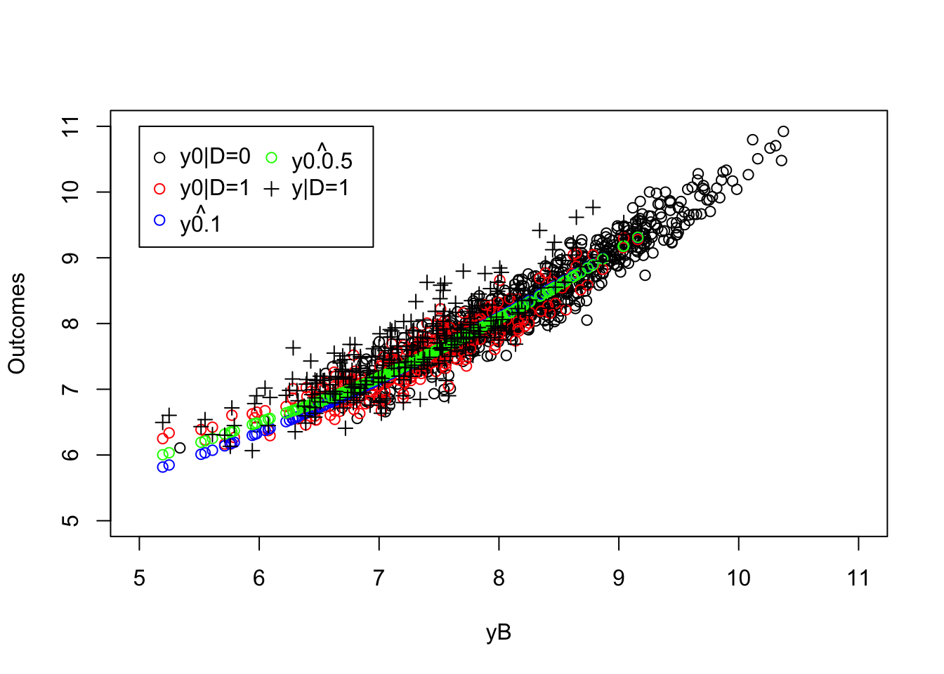

Figure 5.4: LLR Matching estimates

The LLR Matching estimate is equal to 0.192 with a bandwidth of \(1\) and to 0.164 with a bandwidth of \(0.5\), while the true value of the parameter in the population is equal to 0.175.

Let us see how this estimator behaves over sample replications:

# LLR matching fnciton
llr.match <- function(y,D,x,bw,kernel){
  y0.llr <- llr(y[D==0],x[D==0],x[D==1],bw=bw,kernel=kernel)
  return(mean(y[D==1]-y0.llr))
}

# Monte Carlos
monte.carlo.llr <- function(s,N,param,bw,kernel){
  set.seed(s)
  mu <- rnorm(N,param["barmu"],sqrt(param["sigma2mu"]))
  UB <- rnorm(N,0,sqrt(param["sigma2U"]))
  yB <- mu + UB 
  YB <- exp(yB)
  Ds <- rep(0,N)
  V <- rnorm(N,0,sqrt(param["sigma2mu"]+param["sigma2U"]))
  Ds[yB+V<=log(param["barY"])] <- 1 
  epsilon <- rnorm(N,0,sqrt(param["sigma2epsilon"]))
  eta<- rnorm(N,0,sqrt(param["sigma2eta"]))
  U0 <- param["rho"]*UB + epsilon
  y0 <- mu +  U0 + param["delta"] + param["gamma"]*(yB-param["baryB"])^2
  alpha <- param["baralpha"]+  param["theta"]*mu + eta
  y1 <- y0+alpha
  Y0 <- exp(y0)
  Y1 <- exp(y1)
  y <- y1*Ds+y0*(1-Ds)
  Y <- Y1*Ds+Y0*(1-Ds)
  ww.llr <- llr.match(y,Ds,yB,bw=bw,kernel=kernel)
  return(ww.llr)
}

simuls.llr.N <- function(N,Nsim,param,bw,kernel){
  simuls.llr <- matrix(unlist(lapply(1:Nsim,monte.carlo.llr,N=N,param=param,bw=bw,kernel=kernel)),nrow=Nsim,ncol=1,byrow=TRUE)
  colnames(simuls.llr) <- c('LLR')
  return(simuls.llr)
}

sf.simuls.llr.N <- function(N,Nsim,param,bw,kernel){
  sfInit(parallel=TRUE,cpus=8)
  sfExport('llr.match','llr')
  sim.llr <- matrix(unlist(sfLapply(1:Nsim,monte.carlo.llr,N=N,param=param,bw=bw,kernel=kernel)),nrow=Nsim,ncol=1,byrow=TRUE)
  sfStop()
  colnames(sim.llr) <- c('LLR')
  return(sim.llr)
}

Nsim <- 1000
#Nsim <- 10
#N.sample <- c(100,1000,10000,100000)
#N.sample <- c(100,1000,10000)
N.sample <- c(100,1000)
#simuls.llr <- lapply(N.sample,simuls.llr.N,Nsim=Nsim,param=param,bw=bw,kernel=kernel)
simuls.llr <- lapply(N.sample,sf.simuls.llr.N,Nsim=Nsim,param=param,bw=bw,kernel=kernel)
names(simuls.llr) <- N.sample

Let us now plot the resulting estimates:

par(mfrow=c(2,2))
for (i in 1:length(simuls.llr)){
  hist(simuls.llr[[i]][,'LLR'],main=paste('N=',as.character(N.sample[i])),xlab=expression(hat(Delta^yLLR)),xlim=c(-0.15,0.55))
  abline(v=delta.y.tt.com.supp(param),col="red")
}

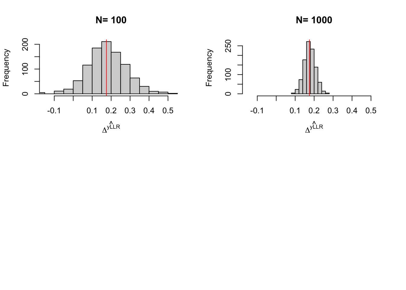
Figure 5.5: Distribution of the \(LLR\) estimator over replications of samples of different sizes

Remark. On key limitation of the LLR Matching estimator that we have studies so far is the fact that it requires the use on only one covariate. What to do when there is more than one covariate? There are basically two solutions. One is to use multidimensional kernels, which are simply products of unidimensionnal kernel functions. In order to make things simpler, we generally standardize variables so that their dimensions are similar. Another approach is to use the propensity score as a dimension reduction device.

5.2.2.1.2 Local Regression Matching on the Propensity Score

The propensity score, which we denote \(P(X_i)\), is the probability that a unit is treated given its observed covariates: \(P(X_i)=\Pr(D_i=1|X_i)\). The key results that enables us to use the propensity score as dimension reduction device has been introduced by Rosenbaum and Rubin (1983):

Theorem 5.7 (Sufficiency of Propensity Score) \((Y_i^1,Y_i^0)\Ind D_i|X_i \Rightarrow (Y_i^1,Y_i^0)\Ind D_i|P(X_i)\).

Proof. \[\begin{align*} \Pr(D_i=1|Y_i^1,Y_i^0,P(X_i)) & = \esp{\Pr(D_i=1|Y_i^1,Y_i^0,X_i)|Y_i^1,Y_i^0,P(X_i)} \\ & = \esp{\Pr(D_i=1|X_i)|Y_i^1,Y_i^0,P(X_i)} \\ & = P(X_i) = \Pr(D_i=1|X_i), \end{align*}\]

where the first equality uses the Law of Iterated Expectations and the second one uses \((Y_i^1,Y_i^0)\Ind D_i|X_i\).

In practice, in order to estimate LLR Matching using the propensity score, you can follow the following steps:

Estimate a logit or probit regression: \(D_i = \uns{\gamma_0 + \gamma_1'X_i + \zeta_i>0}\) (you might use series or splines to be more non-parametric here)
Compute the predicted values (which are estimates of the propensity score): \(\hat{P}(X_i)\) (you could also directly use multivariate non-parametric regression at this stage)
Use \(\hat{P}(X_i)\) as control variable in LLR Matching.

Example 5.8 Let’s see how this works in our example.

First, we need to estimate the propensity score. We are going to use a probit estimator, but things would be much similar with a logit. The most important assumption is the linearity of the link function.

probit.Ds <- glm(Ds~yB, family=binomial(link="probit"))
pscore <- predict(probit.Ds,type="response")

Let us now see how the propensity score looks like as a function of \(y_i^B\):

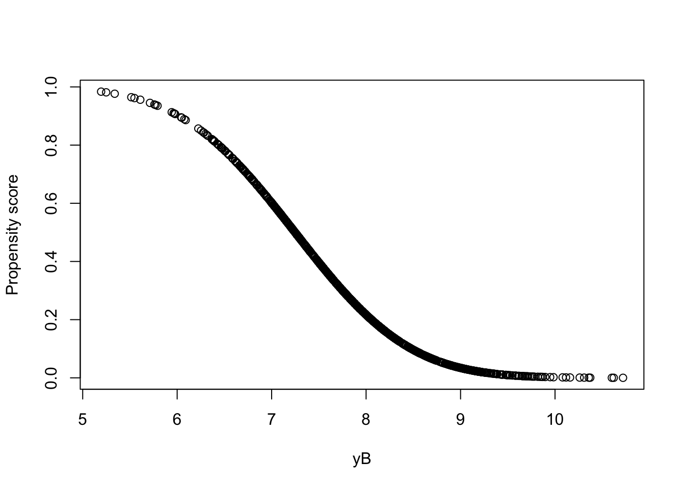
plot(yB,pscore, xlab="yB", ylab="Propensity score")

Figure 5.6: Propensity score as a function of \(y_i^B\)

Let us now compute the LLR Matching estimator using the propensity score.

bw <- 0.1
# run LLR on the untreated sample using treated points as grid points
y0.llr.pscore.0.1 <- llr(y[Ds==0],pscore[Ds==0],pscore[Ds==1],bw=bw,kernel=kernel)    
# compute TT
ww.llr.pscore.0.1 <- llr.match(y,Ds,pscore,bw=bw,kernel=kernel)

Let’s see how the LLR estimator using the propensity score works:

plot(pscore[Ds==0],y[Ds==0], ylab="Outcomes", xlab="Propensity score",xlim=c(0,1),ylim=c(5,12))
points(pscore[Ds==1],y[Ds==1],pch=3,col='blue')
points(pscore[Ds==1],y0[Ds==1],pch=1,col='red')
points(pscore[Ds==1],y0.llr.pscore.0.1,col='green')
legend(0.7,11,c('y0|D=0','y1|D=1','y0|D=1',expression(hat(y0.0.1))),pch=c(1,3,1,1),col=c('black','blue','red','green'),ncol=1)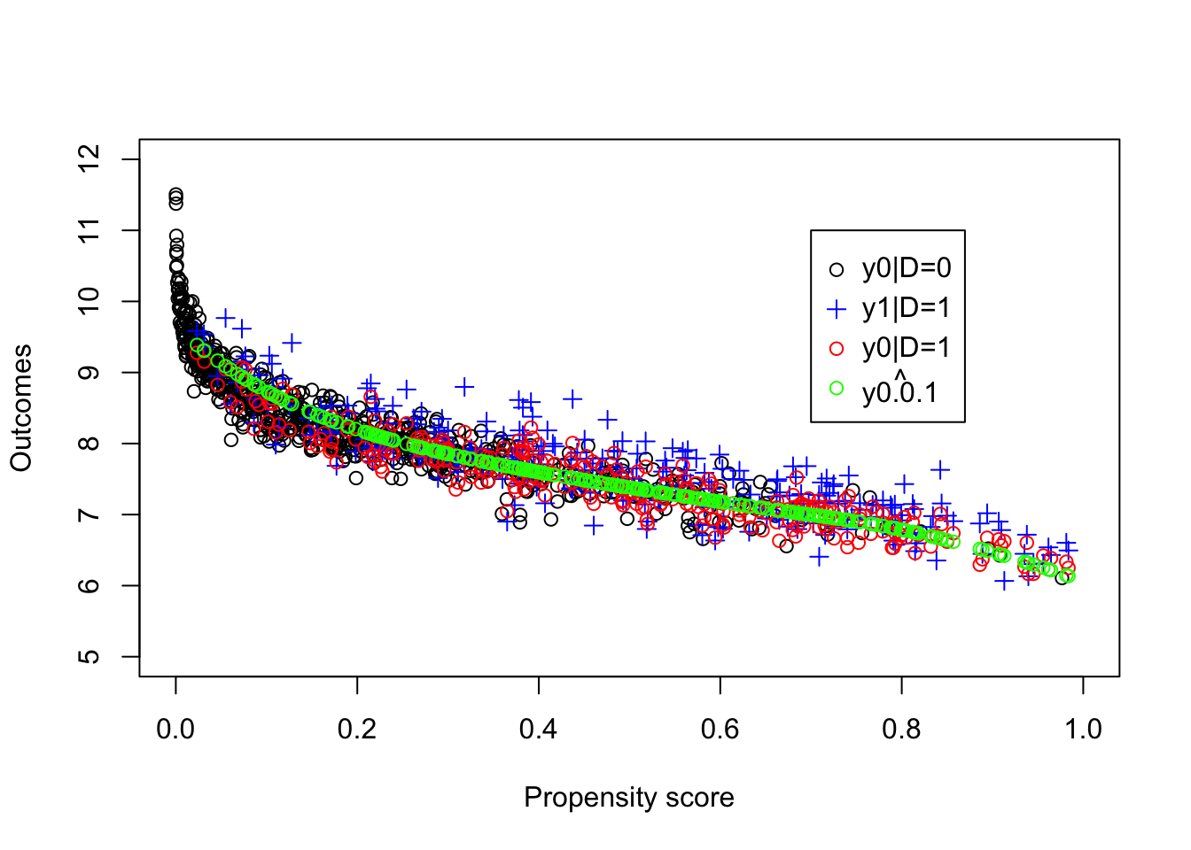

Figure 5.7: Propensity score and potential outcomes

The estimated value of the \(TT\) parameter using LLR Matching on the propensity score is equal to 0.139. Remember that the LLR Matching estimate using \(y_i^B\) directly is equal to 0.192 with a bandwidth of \(1\) and to 0.164 with a bandwidth of \(0.5\), while the true value of the parameter in the population is equal to 0.175.

Remark. We have not seen how to choose the bandwidth optimally. A second thing we are missing is what to do when the density of the pscore is too low and the common support assumption almost does not hold.

5.2.2.1.3 Bandwidth choice

Choosing a bandwidth can be done using one of two approaches. The smaller the bandwidth, the less biased the estimate is, but also the more noisy. With a larger bandwidth, bias increases, but noise decreases. This is the usual Bias/Variance trade-off in nonparametric estimation. Frolich (2005) derives formulae based on the asymptotic distribution of the LLR Matching estimator to help choose the optimal bandwidth. The problem is that these formulae are complex and they are not very precise (the criteria is flat in the bandwidth).

In general, we thus prefer to use use Cross-Validation. Cross validation estimates the MSE using leave-one out estimation and searches for the bandwidth having the lower MSE. Galdo, Smith and Black (2008) suggest to weighted the MSE search by importance of the treated.

Example 5.9 Let’s see how this works in our example.

Let us first (re)define a function to compute the MSE and then compute is:

Let us now plot the link between bandwidth and MSE and what the prediction looks like:

plot(MSE.grid.pscore[1:10],MSE.pscore[1:10], xlab="Bandwidth", ylab="MSE")

plot(pscore[Ds==0],y[Ds==0], ylab="Outcomes", xlab="Propensity score",xlim=c(0,1),ylim=c(5,12))
points(pscore[Ds==1],y[Ds==1],pch=3,col='blue')
points(pscore[Ds==1],y0[Ds==1],pch=1,col='red')
points(pscore[Ds==1],y0.llr.pscore.0.1,col='green')
points(pscore[Ds==1],y0.llr.pscore.bw,col='blue')
legend(0.7,11,c('y0|D=0','y1|D=1','y0|D=1',expression(hat(y0.0.1)),expression(hat(y0.bw))),pch=c(1,3,1,1,1),col=c('black','blue','red','green','blue'),ncol=2)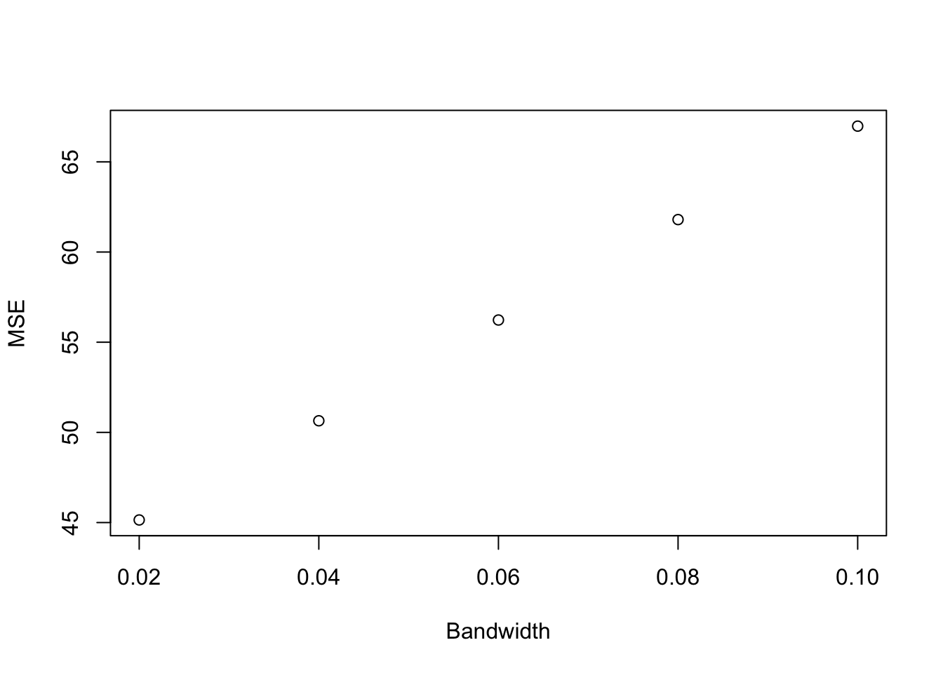

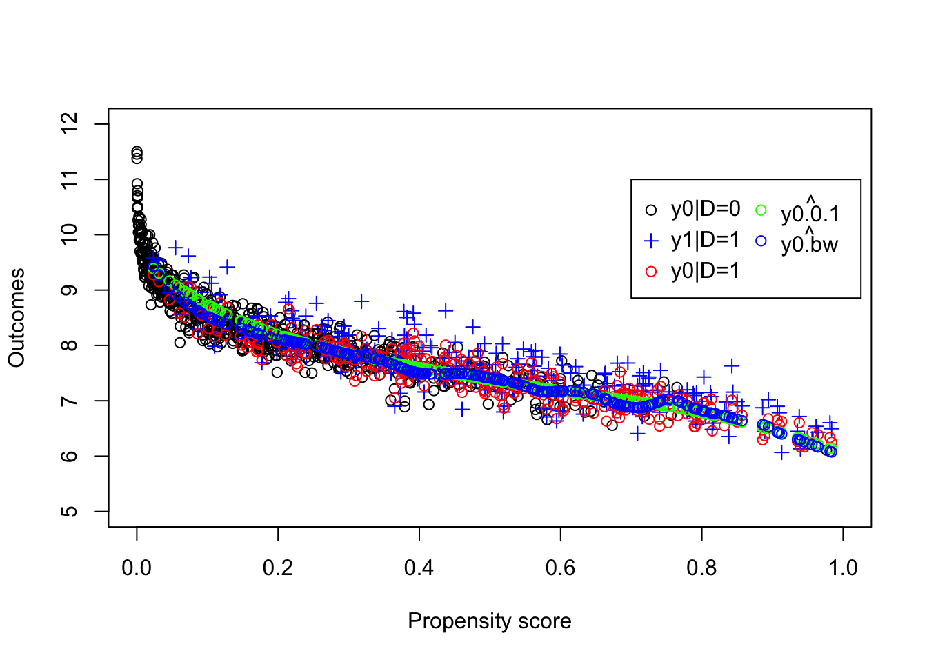
Figure 5.8: LLR Matching on the propensity score with an optimal bandwidth

With the optimal bandwidth, the estimated value of the \(TT\) parameter using LLR Matching on the propensity score is equal to 0.17. Remember that the LLR Matching on the propensity score estimate using a bandwidth of \(0.1\) is equal to 0.139. Using LLR Matching on \(y_i^B\) directly, the estimated \(TT\) is equal to 0.192 with a bandwidth of \(1\) and to 0.164 with a bandwidth of \(0.5\), while the true value of the parameter in the population is equal to 0.175.

5.2.2.1.4 Trimming

Trimming is done to prevent areas where the density of the propensity score is low (where there are very few untreated observations) to blow up our estimates. This is a way to enforce the common support assumption. Note that at the same time we are changing the parameter estimate from \(TT\) to \(TT\) on the trimmed common support.

Trimming, as done for example by Smith and Todd (2005)), goes as follows:

Estimate conditional density \(\hat{f}_{P(X)|D=0}\), for \(i\in\mathcal{I}_1\)
Get rid of observations with density lower than the \(t^{\text{th}}\) percentile of \(\hat{f}_{P(X)|D=0}\), where \(t\) is the trimming level (5% in general).

In order to estimate the density of the propensity score, we use a kernel estimator:

\[\begin{align*} \hat{f}_{P(X)|D=d}(P(X_i)) &= \frac{1}{N_dh}\sum^{N_d}_{j=1}K\left(\frac{P(X_i)-P(X_j)}{h}\right) \\ \hat{S} & = \begin{cases} 1 & \text{ if } \hat{f}_{P(X)|D=0}(P(X_i))>\text{quantile}_{t}(\hat{f}_{P(X)|D=1}(P(X_i))) \\ 0 & \text{ if } \hat{f}_{P(X)|D=0}(P(X_i))\leq\text{quantile}_{t}(\hat{f}_{P(X)|D=1}(P(X_i))), \end{cases} \end{align*}\]

where \(h\) is a different bandwidth that the one chosen for LLR. It can be choosen by using Silverman’s rule of thumb, for example.

Example 5.10 Let us illustrate how this works in our numerical example.

First, let’s define a function to estimate the density and then compute the common support.

# density function estimated at one point
dens.fun.point <- function(n,x,gridx,bw,kernel){
  return(density(x,n=1,from=gridx[n],to=gridx[n],bw=bw,kernel=kernel)[[2]])
}

dens.fun <- function(x,gridx,bw,kernel){
  return(sapply(1:length(gridx), dens.fun.point, x=x, gridx=gridx, bw=bw, kernel=kernel))
}
dens.pscore.D0 <- dens.fun(pscore[Ds==0],pscore[Ds==1],bw=bw.nrd(pscore[Ds==0]),kernel='b')
dens.pscore.D1 <- dens.fun(pscore[Ds==1],pscore[Ds==1],bw=bw.nrd(pscore[Ds==1]),kernel='b')

com.supp <- function(x,gridx,t,bw,kernel){
  dens.x <- dens.fun(x=x,gridx=gridx,bw=bw,kernel=kernel)
  return(ifelse(dens.x<=quantile(dens.x,t),0,1))
}

t<- 0.05
com.supp.pscore <- com.supp(pscore[Ds==0],pscore[Ds==1],t=t,bw=bw.nrd(pscore[Ds==0]),kernel='b')

# estimation using common support and trimming
llr.match.trim <- function(y,D,x,t,bw,kernel){
  com.supp.x <- com.supp(x[D==0],x[D==1],t=t,bw=bw.nrd(x[D==0]),kernel='b')
  y0.llr <- llr(y[D==0],x[D==0],x[D==1][com.supp.x==1],bw=bw,kernel=kernel)
  return(mean(y[D==1][com.supp.x==1]-y0.llr))
}
ww.llr.pscore.trim <- llr.match.trim(y,Ds,pscore,t=t,bw=bw,kernel=kernel)

Let us now plot what the common support looks like:

par(mar=c(5,4,4,5))
plot(pscore[Ds==1],dens.pscore.D0,pch=1,xlim=c(0,1),xlab="Propensity score",ylab="density")
points(pscore[Ds==1],dens.pscore.D1,pch=3)
legend(0.65,2.5,c('fP(yB)|D=0','fP(yB)|D=1','Common Support'),pch=c(1,3,2),col=c('black','black','red'),ncol=1)
par(new=TRUE)
plot(pscore[Ds==1],com.supp.pscore,pch=2,col='red',xlim=c(0,1),ylim=c(0,1),xaxt="n",yaxt="n",xlab="",ylab="")
axis(4)
mtext("Common Support",side=4,line=3)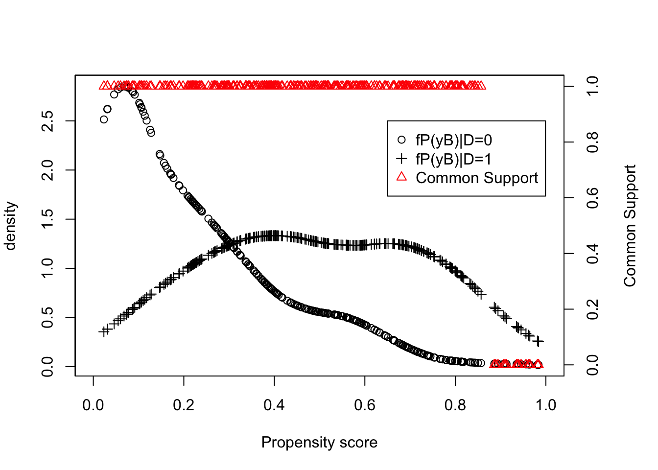

Figure 5.9: Trimming and Common Support

With trimming and the optimal bandwidth, the estimated value of the \(TT\) parameter using LLR Matching on the propensity score is equal to 0.168. Remember that the LLR Matching on the propensity score estimate using the optimal bandwidth but no trimming is equal to 0.17. Using LLR Matching on \(y_i^B\) directly, the estimated \(TT\) is equal to 0.192 with a bandwidth of \(1\) and to 0.164 with a bandwidth of \(0.5\), while the true value of the parameter in the population is equal to 0.175.

Let us run Monte Carlo simulations for this estimator:

monte.carlo.llr.trim <- function(s,N,param,t,bw,kernel){
  set.seed(s)
  mu <- rnorm(N,param["barmu"],sqrt(param["sigma2mu"]))
  UB <- rnorm(N,0,sqrt(param["sigma2U"]))
  yB <- mu + UB 
  YB <- exp(yB)
  Ds <- rep(0,N)
  V <- rnorm(N,0,sqrt(param["sigma2mu"]+param["sigma2U"]))
  Ds[yB+V<=log(param["barY"])] <- 1 
  epsilon <- rnorm(N,0,sqrt(param["sigma2epsilon"]))
  eta<- rnorm(N,0,sqrt(param["sigma2eta"]))
  U0 <- param["rho"]*UB + epsilon
  y0 <- mu +  U0 + param["delta"] + param["gamma"]*(yB-param["baryB"])^2
  alpha <- param["baralpha"]+  param["theta"]*mu + eta
  y1 <- y0+alpha
  Y0 <- exp(y0)
  Y1 <- exp(y1)
  y <- y1*Ds+y0*(1-Ds)
  Y <- Y1*Ds+Y0*(1-Ds)
  probit.Ds <- glm(Ds~yB, family=binomial(link="probit"))
  pscore <- predict(probit.Ds,type="response")
  ww.llr <- llr.match.trim(y,Ds,pscore,t=t,bw=bw,kernel=kernel)
  return(ww.llr)
}

simuls.llr.trim.N <- function(N,Nsim,param,t,bw,kernel){
  simuls.llr.trim <- matrix(unlist(lapply(1:Nsim,monte.carlo.llr.trim,N=N,param=param,t=t,bw=bw,kernel=kernel)),nrow=Nsim,ncol=1,byrow=TRUE)
  colnames(simuls.llr.trim) <- c('LLR Trim')
  return(simuls.llr.trim)
}

sf.simuls.llr.trim.N <- function(N,Nsim,param,t,bw,kernel){
  sfInit(parallel=TRUE,cpus=8)
  sfExport('llr.match.trim','llr','dens.fun.point','dens.fun','com.supp')
  sim.llr.trim <- matrix(unlist(sfLapply(1:Nsim,monte.carlo.llr.trim,N=N,param=param,t=t,bw=bw,kernel=kernel)),nrow=Nsim,ncol=1,byrow=TRUE)
  sfStop()
  colnames(sim.llr.trim) <- c('LLR Trim')
  return(sim.llr.trim)
}

Nsim <- 1000
#Nsim <- 10
#N.sample <- c(100,1000,10000,100000)
#N.sample <- c(100,1000,10000)
N.sample <- c(100,1000)
#N.sample <- c(100)
#simuls.llr.trim <- lapply(N.sample,simuls.llr.trim.N,Nsim=Nsim,param=param,t=t,bw=bw,kernel=kernel)
simuls.llr.trim <- lapply(N.sample,sf.simuls.llr.trim.N,Nsim=Nsim,param=param,t=t,bw=bw,kernel=kernel)
names(simuls.llr.trim) <- N.sample

Let’s plot the resulting distribution (note that we have not chosen the bandwidth optimally in these simulations):

par(mfrow=c(2,2))
for (i in 1:length(simuls.llr.trim)){
  hist(simuls.llr.trim[[i]][,'LLR Trim'],main=paste('N=',as.character(N.sample[i])),xlab=expression(hat(Delta^yLLRTrim)),xlim=c(-0.15,0.55))
  abline(v=delta.y.tt.com.supp(param),col="red")
}

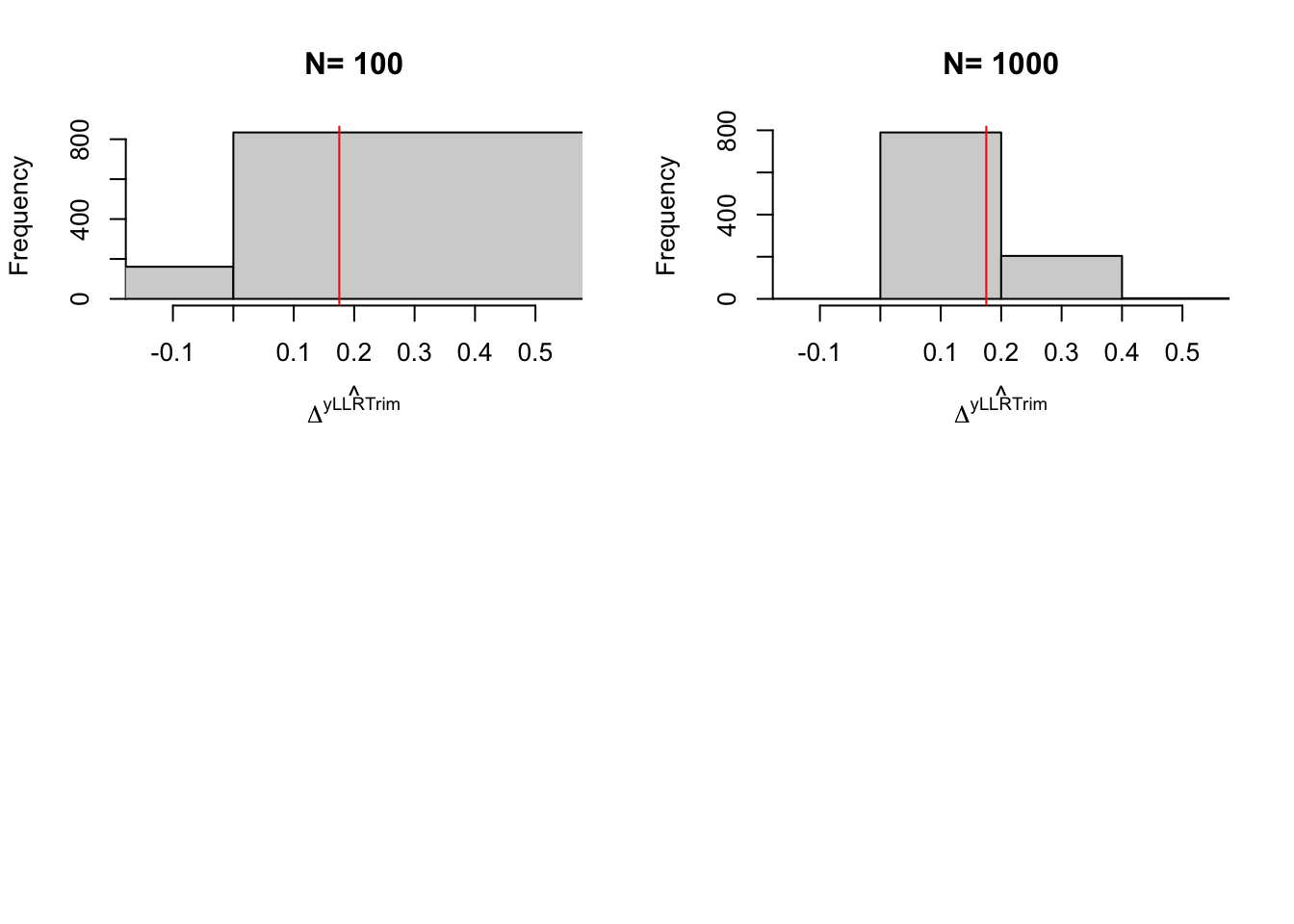
Figure 5.10: Distribution of the trimmed \(LLR\) estimator over replications of samples of different sizes

5.2.2.2 Nearest neighbor matching

With Nearest Neighbor Matching (NNM), we choose the \(M\) closest untreated units for each treated observation \(i\) on the common support, we compute the average outcome of the \(M\) twins to be the imputed counterfactual mean for unit \(i\), take the difference with the observed outcome for \(i\), \(Y_i\), and we take the average of this difference over all treated \(i\) on the common support to obtain the treatment effect estimate:

The \(m^{\text{th}}\) closest neighbor is defined as follows: \[ j_m(i) = \left\{j:D_j=1-D_i \text{ } \&\sum_{k:D_k=1-D_i}\uns{d(i,k)\leq d(i,j)}=m\right\} \] 2. The set of \(M\) closest neighbors is thus: \[ \mathcal{J}_M(i) = \left\{j_1(i),\dots,j_M(i)\right\} \] 3. The number of times observation \(j\) is used as a neighbor (when matching is with replacement) is: \[ \mathcal{K}_M(j) = \sum_{i=1}^N\uns{j\in\mathcal{J}_M(i)}. \]
\(M\) nearest-neighbors pair matching with replacement has the following weights: \[ w_{i,j} = \begin{cases} \frac{1}{M} & \text{ if } j\in\mathcal{J}_M(i)\\ 0 & \text{ if } j\notin\mathcal{J}_M(i) \end{cases} \] 5. We can rewrite the estimator of \(M\) nearest-neighbors matching with replacement as follows:

\[\begin{align*} \hat{\Delta}^Y_{NNM} & = \frac{1}{N_1^S}\sum_{i\in\mathcal{I}^1\cap S}\left(Y_i-\sum_{j\in\mathcal{I}^0}w_{i,j}Y_j\right)\\ & = \frac{1}{N_1^S}\sum_{i\in S}\left(D_i-(1-D_i)\frac{\mathcal{K}_M(i)}{M}\right)Y_i \end{align*}\]

A key issue with how we have implemented NNM is the choice of the metric \(d(i,j)\). Several can be used among the following:

Euclidean distance \[ d(i,j) = \sqrt{\sum_k(X^k_i-X^k_j)^2} \] 2. Normalized Euclidean distance \[ d(i,j) = \sqrt{\sum_k\frac{(X^k_i-X^k_j)^2}{\var{X^k}}} \] 3. Mahalanobis distance \[ d(i,j) = \sqrt{(X-\bar{X})'S^{-1}(X-\bar{X})} \] with \(S\) the covariance matrix of \(X\) 4. Propensity score distance \[ d(i,j) = \sqrt{(P(X_i)-P(X_j))^2}= \left|P(X_i)-P(X_j)\right| \] 5. Genetic distance (Sekhon)

Remark. When \(d(i,k)\leq d(i,j)\) we break ties at random to maintain the integrity of NNM definition.

Remark. Euclidean distance is a bad choice for matching since it gives mucg more weight to covariates observed on a large scale. You are much better off using Normalized Euclidean distance or Mahalanobis distance.

Example 5.11 Let’s see how Nearest Neighbor Matching can be implemented in our example.

The two R packages that can be used for implementing NNM estimators are Matching by Jasjeet Sekhon and MatchIt by Ho, Imai, King and Stuart. As MatchIt is more general and includes most Matching options, I’ll focus on MatchIt.

# building a dataset with treatment, control and outcome
match.data <- data.frame(y=y,Ds=Ds,yB=yB)
# NNM with euclidean distance and 1 to 1 matching with replacement
# selecting the neighbors
nnm.euclid.1.1 <- matchit(Ds~yB,ratio=1,method="nearest",distance='euclidean',replace=TRUE,data=match.data)
# generating the data with neighbors and weights
data.nnm.euclid.1.1 <- match.data(nnm.euclid.1.1)
# estimating tt on the matched data using the weights
tt.nnm.euclid.1.1 <- coef(lm(y~Ds,data=data.nnm.euclid.1.1,weights=weights))[[2]]

# NNM with euclidean distance and 5 to 1 matching with replacement
# selecting the neighbors
nnm.euclid.5.1 <- matchit(Ds~yB,ratio=5,method="nearest",distance='euclidean',replace=TRUE,data=match.data)
# generating the data with neighbors and weights
data.nnm.euclid.5.1 <- match.data(nnm.euclid.5.1)
# estimating tt on the matched data using the weights
tt.nnm.euclid.5.1 <- coef(lm(y~Ds,data=data.nnm.euclid.5.1,weights=weights))[[2]]

# NNM with propensity score distance and 1 to 1 matching with replacement
# selecting the neighbors
nnm.pscore.1.1 <- matchit(Ds~yB,ratio=1,method="nearest",distance='glm',link='probit',replace=TRUE,data=match.data)
# generating the data with neighbors and weights
data.nnm.pscore.1.1 <- match.data(nnm.pscore.1.1)
# estimating tt on the matched data using the weights
tt.nnm.pscore.1.1 <- coef(lm(y~Ds,data=data.nnm.pscore.1.1,weights=weights))[[2]]

# NNM with propensity score distance and 5 to 1 matching with replacement
# selecting the neighbors
nnm.pscore.5.1 <- matchit(Ds~yB,ratio=5,method="nearest",distance='glm',link='probit',replace=TRUE,data=match.data)
# generating the data with neighbors and weights
data.nnm.pscore.5.1 <- match.data(nnm.pscore.5.1)
# estimating tt on the matched data using the weights
tt.nnm.pscore.5.1 <- coef(lm(y~Ds,data=data.nnm.pscore.5.1,weights=weights))[[2]]

# NNM with Mahalanobis distance and 1 to 1 matching with replacement
# selecting the neighbors
nnm.maha.1.1 <- matchit(Ds~yB,ratio=1,method="nearest",distance='mahalanobis',replace=TRUE,data=match.data)
# generating the data with neighbors and weights
data.nnm.maha.1.1 <- match.data(nnm.maha.1.1)
# estimating tt on the matched data using the weights
tt.nnm.maha.1.1 <- coef(lm(y~Ds,data=data.nnm.maha.1.1,weights=weights))[[2]]

# NNM with Mahalanobis distance and 5 to 1 matching with replacement
# selecting the neighbors
nnm.maha.5.1 <- matchit(Ds~yB,ratio=5,method="nearest",distance='mahalanobis',replace=TRUE,data=match.data)
# generating the data with neighbors and weights
data.nnm.maha.5.1 <- match.data(nnm.maha.5.1)
# estimating tt on the matched data using the weights
tt.nnm.maha.5.1 <- coef(lm(y~Ds,data=data.nnm.maha.5.1,weights=weights))[[2]]

The estimates are going to be pretty similar among all the methods in our example. For example, 5 to 1 NNM with the Mahalanobis distance yields an estimate of \(TT\) of 0.147.

The MatchIt package offers some pretty cool visualization tools. For example, we can visualize the standardized distance (mean difference in units of standard deviation) between the treated and control units before and after matching, and the distribution of covariates before and after matching:

# plot of standardized distance
plot(summary(nnm.euclid.1.1),xlim=c(0,2))

# plot of distribution of covariates
plot(nnm.euclid.1.1, type = "density", interactive = FALSE)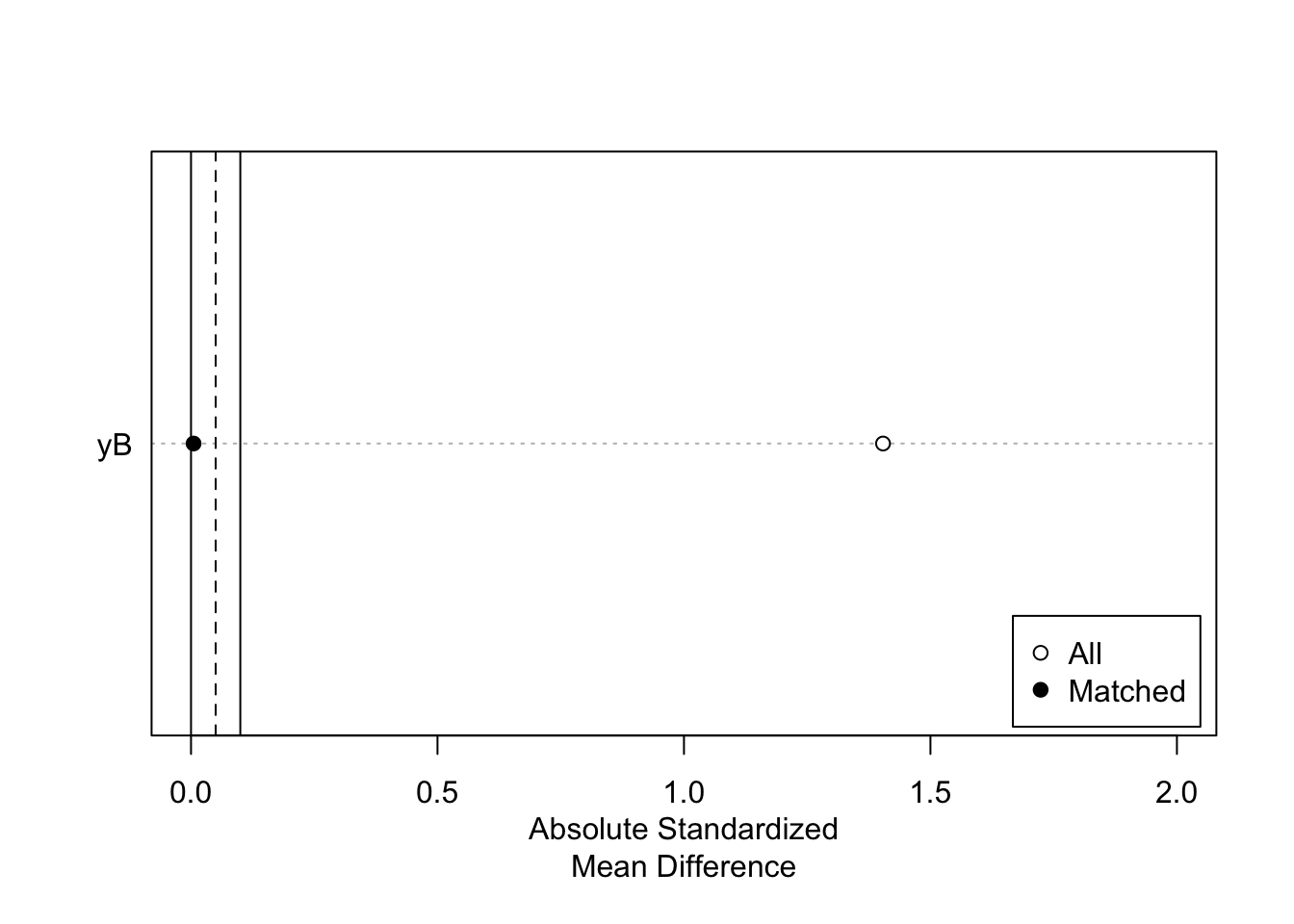

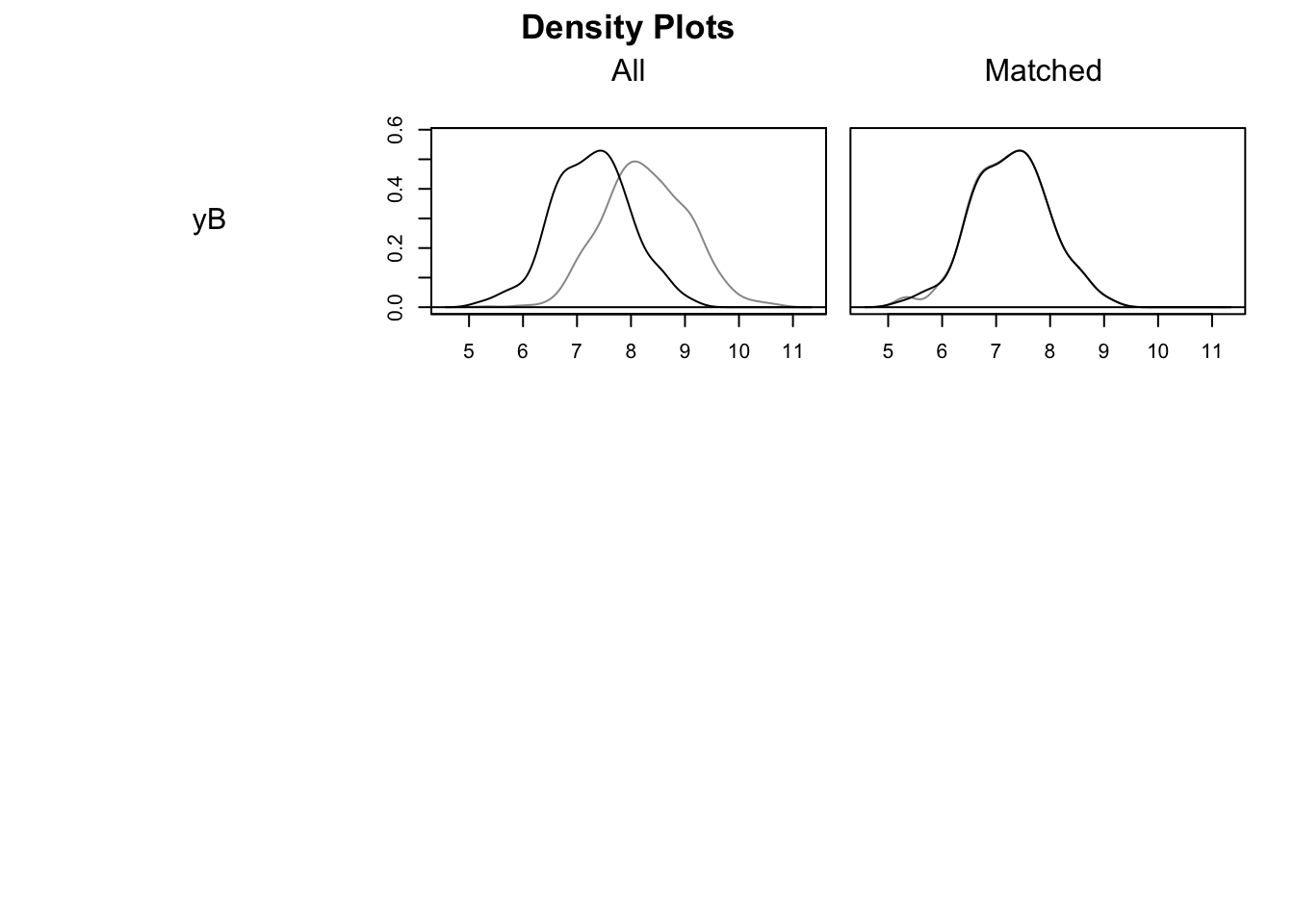
Figure 5.11: Trimming and Common Support

As Figure 5.11 shows, the Matching procedure is pretty effective in that it completely aligns treated and control units in terms of the pre-treatment covariate. MatchIt is much reacher than I can do it justice here. See its amazing documentation for inspiration and guidance.

Let us run Monte Carlo simulations for this estimator:

monte.carlo.nnm <- function(s,N,param,...){
  set.seed(s)
  mu <- rnorm(N,param["barmu"],sqrt(param["sigma2mu"]))
  UB <- rnorm(N,0,sqrt(param["sigma2U"]))
  yB <- mu + UB 
  YB <- exp(yB)
  Ds <- rep(0,N)
  V <- rnorm(N,0,sqrt(param["sigma2mu"]+param["sigma2U"]))
  Ds[yB+V<=log(param["barY"])] <- 1 
  epsilon <- rnorm(N,0,sqrt(param["sigma2epsilon"]))
  eta<- rnorm(N,0,sqrt(param["sigma2eta"]))
  U0 <- param["rho"]*UB + epsilon
  y0 <- mu +  U0 + param["delta"] + param["gamma"]*(yB-param["baryB"])^2
  alpha <- param["baralpha"]+  param["theta"]*mu + eta
  y1 <- y0+alpha
  Y0 <- exp(y0)
  Y1 <- exp(y1)
  y <- y1*Ds+y0*(1-Ds)
  Y <- Y1*Ds+Y0*(1-Ds)
  # building a dataset with treatment, control and outcome
  match.data <- data.frame(y=y,Ds=Ds,yB=yB)
  # NNM with euclidean distance and 1 to 1 matching with replacement
  # selecting the neighbors
  nnm.euclid.1.1 <- matchit(Ds~yB,data=match.data,...)
  # generating the data with neighbors and weights
  data.nnm.euclid.1.1 <- match.data(nnm.euclid.1.1)
  # estimating tt on the matched data using the weights
  tt.nnm.euclid.1.1 <- coef(lm(y~Ds,data=data.nnm.euclid.1.1,weights=weights))[[2]]
  return(tt.nnm.euclid.1.1)
}

simuls.nnm.N <- function(N,Nsim,param,...){
  simuls.nnm <- matrix(unlist(lapply(1:Nsim,monte.carlo.nnm,N=N,param=param,...)),nrow=Nsim,ncol=1,byrow=TRUE)
  colnames(simuls.nnm) <- c('NNM')
  return(simuls.nnm)
}

sf.simuls.nnm.N <- function(N,Nsim,param,...){
  sfInit(parallel=TRUE,cpus=8)
  sfLibrary(MatchIt)
  sim.nnm <- matrix(unlist(sfLapply(1:Nsim,monte.carlo.nnm,N=N,param=param,...)),nrow=Nsim,ncol=1,byrow=TRUE)
  sfStop()
  colnames(sim.nnm) <- c('NNM')
  return(sim.nnm)
}

Nsim <- 1000
#Nsim <- 10
#N.sample <- c(100,1000,10000,100000)
#N.sample <- c(100,1000,10000)
N.sample <- c(100,1000)
#N.sample <- c(100)
#simuls.nnm <- lapply(N.sample,simuls.nnm.N,Nsim=Nsim,param=param,ratio=1,method="nearest",distance='euclidean',replace=TRUE)
simuls.nnm <- lapply(N.sample,sf.simuls.nnm.N,Nsim=Nsim,param=param,ratio=1,method="nearest",distance='euclidean',replace=TRUE)
names(simuls.nnm) <- N.sample

Let’s plot the resulting distribution (note that we have not chosen the bandwidth optimally in these simulations):

par(mfrow=c(2,2))
for (i in 1:length(simuls.nnm)){
  hist(simuls.nnm[[i]][,'NNM'],main=paste('N=',as.character(N.sample[i])),xlab=expression(hat(Delta^yNNM)),xlim=c(-0.15,0.55))
  abline(v=delta.y.tt.com.supp(param),col="red")
}

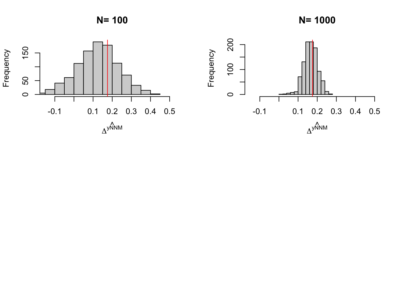
Figure 5.12: Distribution of the NNM estimator over replications of samples of different sizes

5.2.2.3 Reweighting matching

Reweighting matching uses the following set of weigths:

\[\begin{align*} w_{i,j} & = \frac{\frac{\hat{P}(X_j)}{1-\hat{P}(X_j)}}{\sum_{j\in\mathcal{I}_0}\frac{\hat{P}(X_j)}{1-\hat{P}(X_j)}} = w_j. \end{align*}\]

Since these weights do not depend on \(i\), we can thus write:

\[\begin{align*} \hat{\Delta}^Y_{TT} & = \frac{1}{N_1}\sum_{i\in\mathcal{I}_1}\left(Y_i-\sum_{j\in\mathcal{I}_0}w_{i,j}Y_j\right)\\ & = \frac{1}{N_1}\sum_{i\in\mathcal{I}_1}Y_i - \sum_{j\in\mathcal{I}_0}w_{j}Y_j \end{align*}\]

The Reweighting estimator is thus very simple and quick: it only needs two separate summations instead of two nested summations.

Example 5.12 Let’s see how the reweighting estimator works in practice.

The main object that we have to build are the weights. They stem directly from the propensity score estimates.

# computing weights
pscore.weights <- (pscore/(1-pscore))*(1-mean(Ds))/mean(Ds)
# get rid of weights for the treated
pscore.weights[Ds==1] <- 0
# normalize by sum of weights for the untreated
pscore.weights <- pscore.weights/sum(pscore.weights)

# counterfactual estimation using reweighting:
y0.D1.reweighting <- weighted.mean(y[Ds==0],w=pscore.weights[Ds==0])
# TT estimation
TT.reweighting <- mean(y[Ds==1])-y0.D1.reweighting

The \(TT\) estimated by the reweighting estimator is equal to 0.297. Remember that the true value of the parameter in the population is equal to 0.175.

Let us run Monte Carlo simulations for this estimator:

monte.carlo.reweight <- function(s,N,param){
  set.seed(s)
  mu <- rnorm(N,param["barmu"],sqrt(param["sigma2mu"]))
  UB <- rnorm(N,0,sqrt(param["sigma2U"]))
  yB <- mu + UB 
  YB <- exp(yB)
  Ds <- rep(0,N)
  V <- rnorm(N,0,sqrt(param["sigma2mu"]+param["sigma2U"]))
  Ds[yB+V<=log(param["barY"])] <- 1 
  epsilon <- rnorm(N,0,sqrt(param["sigma2epsilon"]))
  eta<- rnorm(N,0,sqrt(param["sigma2eta"]))
  U0 <- param["rho"]*UB + epsilon
  y0 <- mu +  U0 + param["delta"] + param["gamma"]*(yB-param["baryB"])^2
  alpha <- param["baralpha"]+  param["theta"]*mu + eta
  y1 <- y0+alpha
  Y0 <- exp(y0)
  Y1 <- exp(y1)
  y <- y1*Ds+y0*(1-Ds)
  Y <- Y1*Ds+Y0*(1-Ds)
  # pscore estimation
  probit.Ds <- glm(Ds~yB, family=binomial(link="probit"))
  pscore <- predict(probit.Ds,type="response")
  # computing weights
  pscore.weights <- pscore/(1-pscore)*(1-mean(Ds))/mean(Ds)
  # get rid of weights for the treated
  pscore.weights[Ds==1] <- 0
  # normalize by sum of weights for the untreated
  pscore.weights <- pscore.weights/sum(pscore.weights)
  # counterfactual estimation using reweighting:
  y0.D1.reweighting <- weighted.mean(y[Ds==0],w=pscore.weights[Ds==0])
  # TT estimation
  TT.reweighting <- mean(y[Ds==1])-y0.D1.reweighting
  return(TT.reweighting)
}

simuls.reweight.N <- function(N,Nsim,param){
  simuls.reweight <- matrix(unlist(lapply(1:Nsim,monte.carlo.reweight,N=N,param=param)),nrow=Nsim,ncol=1,byrow=TRUE)
  colnames(simuls.reweight) <- c('Reweighting Matching')
  return(simuls.reweight)
}

sf.simuls.reweight.N <- function(N,Nsim,param){
  sfInit(parallel=TRUE,cpus=8)
  sim.reweight <- matrix(unlist(sfLapply(1:Nsim,monte.carlo.reweight,N=N,param=param)),nrow=Nsim,ncol=1,byrow=TRUE)
  sfStop()
  colnames(sim.reweight) <- c('Reweighting Matching')
  return(sim.reweight)
}

Nsim <- 1000
#Nsim <- 10
#N.sample <- c(100,1000,10000,100000)
#N.sample <- c(100,1000,10000)
N.sample <- c(100,1000)
#N.sample <- c(100)
#simuls.reweight <- lapply(N.sample,simuls.reweight.N,Nsim=Nsim,param=param)
simuls.reweight<- lapply(N.sample,sf.simuls.reweight.N,Nsim=Nsim,param=param)
names(simuls.reweight) <- N.sample

Let’s plot the resulting distribution (note that we have not chosen the bandwidth optimally in these simulations):

par(mfrow=c(2,2))
for (i in 1:length(simuls.reweight)){
  hist(simuls.reweight[[i]][,'Reweighting Matching'],main=paste('N=',as.character(N.sample[i])),xlab=expression(hat(Delta^yReweight)),xlim=c(-0.15,0.55))
  abline(v=delta.y.tt.com.supp(param),col="red")
}

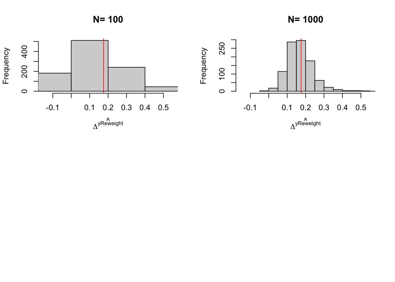
Figure 5.13: Distribution of the Reweighting Matching estimator over replications of samples of different sizes

5.2.2.4 Doubly robust matching

Doubly robust matching combines regression adjusted matching and weighting matching. Its main property is that it is robust to misspecification of the regression functions for the outcomes or for the treatment: even if one of these functions is misspecified, the doubly robust matching estimator will be consistent as long as the other one is correctly specified.

TO DO

5.2.3 Estimating precision

There are several ways to estimate of the precision of matching estimators. In practice, we end up using the bootstrap for LLR, reweighting and doubly robust matching and to use CLT-based approximations for NNM. This is because of the combination of several factors:

The bootstrap is inconsistent for NNM: Abadie and Imbens (2008) show that the bootstrap fails to approximate the distribution of the NNM estimator.
The CLT-based formulae for LLR and reweighting matching are in general difficult to compute or take too much time to run, or are attached to specific estimators.
The CLT-based formula developped by Abadie and Imbens (2006) for NNM are simple to compute.

Here, we are going to first give a sense of the maximum possible precision of matching estimators. Then we will see how this result applies to teh CLT-based formulae for LLR and reweighting matching. We will then describe the CLT-based formulae for NNM.

5.2.3.1 Maxium precision of matching estimators

The maximum level of precision that any estimator relying on the matching assumptions can hope to reach is the minimum asymptotic variance that any such estimator cannot get under. The derivation of this bound (called the semiparametric efficiency bound of matching estimators) is due to Hahn (1998).

Theorem 5.8 (Efficiency Bound under Conditional Independence) Under Assumption 5.2, we have, for all consistent estimators \(\hat{\Delta^Y_{ATE}}\) and \(\hat{\Delta^Y_{TT}}\) of \(\Delta^Y_{ATE}\) and \(\Delta^Y_{TT}\):

\[\begin{align*} \asym\var{\hat{\Delta^Y_{ATE}}} & \geq \frac{1}{N}\esp{\frac{\var{Y_i^1|X_i}}{\Pr(D_i=1|X_i)}+\frac{\var{Y_i^0|X_i}}{1-\Pr(D_i=1|X_i)}+(\Delta^Y_{ATE}(X_i)-\Delta^Y_{ATE})^2} \\ \asym\var{\hat{\Delta^Y_{TT}}} & \geq \frac{1}{N}\esp{\frac{\Pr(D_i=1|X_i)\var{Y_i^1|X_i}}{\Pr(D_i=1)}+\frac{\Pr(D_i=1|X_i)^2\var{Y_i^0|X_i}}{\Pr(D_i=1)(1-\Pr(D_i=1|X_i))}}\\ & \phantom{\geq} +\frac{1}{N}\esp{\frac{(\Delta^Y_{TT}(X_i)-\Delta^Y_{TT})^2\Pr(D_i=1|X_i)}{\Pr(D_i=1)}}. \end{align*}\]

Proof. See Hahn (1998).

Theorem 5.8 enables to compute a lower bound on the variance of any matching estimator. Moreover, if it can be shown that a given estimator reaches the semi-parametric efficiency bound (i.e. is efficient), then Theorem 5.8 enables to compute its precision using a CLT-based approximation (and not only a lower bound).

There are thus two key issues with using Theorem 5.8 in practice:

Is it the case that our candidate matching estimator is efficient?
How can we operationalize the formula in Theorem 5.8?

Question 1 is a theoretical question about properties of estimators while question 2 is a practical question. Theorem 5.8 shows that estimating the variance of efficient matching estimators requires to estimate the propensity score, but also two conditional variance terms and the conditional treatment on the treated parameter. Thus Theorem 5.8 requires the estimation of multiple nonparametric functions. It might sometimes be preferable to rey on the bootstrap, if the bootstrap is consistent (which it is when the estimator is efficient, hence the relevance of question 1).

5.2.3.2 Estimating precision of LLR and reweighting matching

It is in general believed that LLR and Reweighting Matching estimators are efficient, and thus that they reach the semi-parametric efficiency bound derived by Hahn (1998). The devil is in the details though, since the particular form of the estimators and the conditions imposed on the d.g.p. are crucial for these results to hold. Let’s state the results that hold for the reweighting and LLR matching estimators.

Theorem 5.9 (Asymptotic Distribution of Reweighting and LLR Matching) Under Assumption 5.2 and technical conditions made clear in Hahn (1998) and Mammen et al (2016), the Reweighting matching estimator and the LLR matching estimator based on the propensity score of the Average Effect of the Treatment on the Treated are consistent, asymptotically normally distributed and reach the nonparametric efficiency bound.

Proof. See Hahn (1998) and Mammen et al (2016).

Remark. Mammen et al (2016) only prove the consistency and efficiency of the LLR matching estimator using the propensity score for the ATE. Extension to the TT is assumed here but should be checked rigorously.

Remark. Heckman et al (1998) derive the distribution of the LLR Matching estimator based on the propensity score, but their derivation does not seem to reach the semiparametric efficiency bound. More investigation is needed to reconcile this result with the one in Mammen et al (2016).

In practice, we do not use CLT-based approximations to estimate the precision of LLR Matching on the propensity score, since these estimators require rather complex computations. We rather rely on the nonparametric bootstrap, we is justified by the existence of the CLT-based results.

Remark. Mammen et al (2016) show that the nonparametric bootstrap can be used to estimate the distribution of LLR matching on the propensity score under technical conditions.

Example 5.13 Let us see how we can use the bootstrap in our example.

Let’s first write a function to generate a bootstrap estimate:

# function for the bootstrap of LLR
bootstrap.llr.trim <- function(s,y,D,x,t,bw,kernel){
  set.seed(s)
  boot.samp <- sample(N,replace=TRUE)
  y.boot <- y[boot.samp]
  D.boot <- D[boot.samp]
  x.boot <- x[boot.samp]
  llr.match.trim.boot <- llr.match.trim(y.boot,D.boot,x.boot,t=t,bw=bw,kernel=kernel)
  return(llr.match.trim.boot)
}  
# function for the bootstrap of Reweighting
bootstrap.reweigthing <- function(s,y,D,x){
  set.seed(s)
  boot.samp <- sample(N,replace=TRUE)
  y.boot <- y[boot.samp]
  D.boot <- D[boot.samp]
  x.boot <- x[boot.samp]
  # pscore estimation
  probit.Ds <- glm(D.boot~x.boot, family=binomial(link="probit"))
  pscore <- predict(probit.Ds,type="response")
  # computing weights
  pscore.weights <- pscore/(1-pscore)*(1-mean(D.boot))/mean(D.boot)
  # get rid of weights for the treated
  pscore.weights[D.boot==1] <- 0
  # normalize by sum of weights for the untreated
  pscore.weights <- pscore.weights/sum(pscore.weights)
  # counterfactual estimation using reweighting:
  y0.D1.reweighting <- weighted.mean(y.boot[D.boot==0],w=pscore.weights[D.boot==0])
  # TT estimation
  TT.reweighting <- mean(y.boot[D.boot==1])-y0.D1.reweighting
  return(TT.reweighting)
}  

# testing
test.boot.llr <- bootstrap.llr.trim(1234,y=y,D=Ds,x=yB,t=t,bw=bw,kernel=kernel)
test.boot.reweight <- bootstrap.reweigthing(1234,y=y,D=Ds,x=yB)

# parallelized computation of bootstrap
sf.boot.llr.N <- function(Nsim,...){
  sfInit(parallel=TRUE,cpus=8)
  sfExport('llr.match.trim','llr','dens.fun.point','dens.fun','com.supp','bootstrap.llr.trim')
  sim.boot.llr <- matrix(unlist(sfLapply(1:Nsim,bootstrap.llr.trim,...)),nrow=Nsim,ncol=1,byrow=TRUE)
  sfStop()
  colnames(sim.boot.llr) <- c('BootLLR')
  return(sim.boot.llr)
}

sf.boot.reweight.N <- function(Nsim,...){
  sfInit(parallel=TRUE,cpus=8)
  sim.boot.reweight <- matrix(unlist(sfLapply(1:Nsim,bootstrap.reweighting,...)),nrow=Nsim,ncol=1,byrow=TRUE)
  sfStop()
  colnames(sim.boot.reweight) <- c('BootReweight')
  return(sim.boot.reweight)
}


t <- 0.05
kernel <- 'gaussian'
N.boot <- 1000
bw <- 0.5
boot.llr <- sapply(1:N.boot,bootstrap.llr.trim,y=y,D=Ds,x=yB,t=t,bw=bw,kernel=kernel)
boot.reweight <- sapply(1:N.boot,bootstrap.reweigthing,y=y,D=Ds,x=yB)

#boot.llr <- sf.boot.llr.N(Nsim=N.boot,y=y,D=Ds,x=yB,t=t,bw=bw,kernel=kernel)
#boot.reweight <- sf.boot.reweight.N(Nsim=N.boot,y=y,D=Ds,x=yB)

#  sfInit(parallel=TRUE,cpus=8)
#  sfExport('llr.match.trim','llr','dens.fun.point','dens.fun','com.supp','bootstrap.llr.trim','y','Ds','yB')
#  sim.boot.reweight <- sfLapply(1:2,bootstrap.llr.trim,y=y,D=Ds,x=yB,t=t,bw=bw,kernel=kernel)
#  sim.boot.reweight <- lapply(1:2,bootstrap.llr.trim,y=y,D=Ds,x=yB,t=t,bw=bw,kernel=kernel)
#  sfStop()

Let’s now compute the precision estimators:

delta <- 0.99
precision.llr <- function(k){
  return(2*quantile(abs(simuls.llr[[k]][,'LLR']-delta.y.tt.com.supp(param)),probs=c(delta)))
}
precision.llr.trim <- function(k){
  return(2*quantile(abs(simuls.llr.trim[[k]][,'LLR Trim']-delta.y.tt.com.supp(param)),probs=c(delta)))
}
precision.reweighting <- function(k){
  return(2*quantile(abs(simuls.reweight[[k]][,'Reweighting Matching']-delta.y.tt.com.supp(param)),probs=c(delta)))
}
precision.nnm <- function(k){
  return(2*quantile(abs(simuls.nnm[[k]][,'NNM']-delta.y.tt.com.supp(param)),probs=c(delta)))
}

precision.nnm.100 <- precision.nnm(1)
precision.nnm.1000 <- precision.nnm(2)
precision.llr.100 <- precision.llr(1)
precision.llr.1000 <- precision.llr(2)
precision.llr.trim.100 <- precision.llr.trim(1)
precision.llr.trim.1000 <- precision.llr.trim(2)
precision.reweighting.100 <- precision.reweighting(1)
precision.reweighting.1000 <- precision.reweighting(2)
precision.llr.trim.boot.1000 <- 2*quantile(abs(boot.llr-delta.y.tt.com.supp(param)),probs=c(delta))
precision.reweighting.boot.1000 <- 2*quantile(abs(boot.reweight-delta.y.tt.com.supp(param)),probs=c(delta))

With 100 obs, the true precision of LLR Matching is 0.61, while it is of 4.81 with trimming and of 0.9 with reweighting. With 1000 observation, the true precision of LLR Matching without trimming is 0.15 and with trimming is 0.3 and the precision of reweighting matching is 0.43. Using the bootstrap with 1000 replications, the estimated precision of LLR with trimming is 0.14 while the estimated precision of reweighting matching is 0.86.

5.2.3.3 Estimating the precision of Nearest Neighbour Matching

Abadie and Imbens (2006) propose a variance estimator for Nearest Neighbor Matching based on the CLT. But before that, Abadie and Imbens (2006) prove several fundamental results on the properties of NNM. They show that NNM is not \(\sqrt{N}\)-consistent for ATE nor for TT. It means that, in general, NNM is affected by a bias term that is larger than \(\frac{1}{\sqrt{N}}\) even when sample size grows large. Fortunately, Abadie and Imbens (2006) show that this bias term goes to zero as sample size grows large, so that NNM is always consistent. They also show that, under reasonable conditions, this bias term goes to zero faster than \(\sqrt{N}\) when the number of untreated units is much larger than the number of treated units. It means that under these conditions, this term can be ignored and the distribution of NNM converges to a standard normal at a \(\sqrt{N}\) rate. They also show that the NNM estimator does not reach the semi-parametric efficiency bound of Theorem 5.8, but they also that the difference between the two variances is smaller than \(\frac{1}{2M}\) where \(M\) is the number of matches used. With NNM on one neighbor, the increase in variance relative to the most efficient estimator is of at most 50%, while with 5 neighbors, the increase in asymptotic variance is of at most 10%. Finally, Abadie and Imbens (2008) show that even when NNM is asymptotically normal and \(\sqrt{N}\)-consistent, the bootstrap might fail to approximate its distribution. Note that the bootstrap recovers its value if we allow the number of matched neighbors to increase with sample size.

So, now, what is the CLT-based estimator for the variance of NNM proposed by Abadie and Imbens (2006)? It is a clever use of the matching method to compute a variance estilmate using pairwise comparisons. Note that this estimator is correct only when NNM is asymptotically normal and \(\sqrt{N}\)-consistent, so when there are many more control than treated observations, or when the number of neighbors is large enough.

Let us first derive the asymptotic distribution of the NNM estimator. We need to assume something about the data generating process (in general that the data are i.i.d.). The assumption needed for NNM to be consistent is slightly more involved and requires restrictions on the ratio of treated to untreated observations \(\frac{N_1}{N_0}\):

Hypothesis 5.8 (i.i.d. distribution for matching) Conditional on \(D_i=d\), the sample consists of independent draws from \(Y,X|D=d\), \(d\in\left\{0,1\right\}\). For some \(r\geq 1\), \(\frac{N^r_1}{N_0}\rightarrow \theta\), with \(0<\theta<\infty\).

Theorem 5.10 (Asymptotic Distribution of NNM) Under Assumptions 5.2, 5.7, 5.8 and Assumption 4 in Abadie and Imbens (2006), we have: \[\begin{align*} \sqrt{N_1}(\hat{\Delta}^Y_{NNM}-\Delta^Y_{TT}) & \stackrel{d}{\rightarrow} \mathcal{N}\left(0,V^{E,TT}+V^{\Delta^Y_{TT}(X)}\right), \end{align*}\] where: \[\begin{align*} V^{E,TT} & = \frac{1}{N_1}\sum_{i=1}^N\left(D_i-(1-D_i)\frac{\mathcal{K}_M(i)}{M}\right)^2\var{Y_i|D_i,X_i}\\ V^{\Delta^Y_{TT}(X)} & = \esp{(\Delta^Y_{TT}(X_i)-\Delta^Y_{TT})^2|D_i=1}. \end{align*}\]

Proof. See Corollary 1 in Abadie and Imbens (2006).

Remark. The general formula for the precision of the NNM estimator is close to all the same estimators we have seen so far: its is a sum of the variance of the outcome conditional on \(X_i\) among the treated and among the untreated weighted by their relative importance in the estimation. In addition, a term reflecting the variance of treatment effects due to \(X_i\) has appeared.

The key to Abadie and Imbens (2006) estimator is to find a way to estimate \(\var{Y_i|D_i,X_i}\). We could use the residuals from linear regressions or from non-parametric regressions, but that would be extremely burdensome. Abadie and Imbens (2006) propose a very clever trick to simplify the estimation of \(\var{Y_i|D_i,X_i}\) by using a variation of the matching estimator. Define \(l_m(i)\) the \(m^{\text{th}}\) closest unit to \(i\) among the units with the same value for the treatment indicator. Abadie and Imbens (2006)’s estimator for \(\var{Y_i|D_i,X_i}\) is:

\[\begin{align*} \hatvar{Y_i|D_i,X_i} & = \frac{J}{J+1}\left(Y_i-\frac{1}{J}\sum_{m=1}^JY_{l_j(i)}\right)^2. \end{align*}\]

Abadie and Imbens (2006) then combine this estimator with an estimator for \(V^{\Delta^Y_{TT}(X)}\) which has to be corrected by the size of the variance of outcomes given \(X_i\). Eventually, after some algebra, we have:

\[\begin{align*} \hat{V}^{E,TT}+\hat{V}^{\Delta^Y_{TT}(X)} & = \frac{1}{N_1}\sum_{i:D_i=1}\left(Y_i-\frac{1}{M}\sum_{j\in\mathcal{J}_M(i)}Y_j-\Delta^Y_{TT}\right)^2 \\ & \phantom{=}+\frac{1}{N_1}\sum_{i=1}^N(1-D_i)\left(\frac{\mathcal{K}_M(i)(\mathcal{K}_M(i)-1)}{M^2}\right)\hatvar{Y_i|D_i,X_i}. \end{align*}\]

Theorem 7 in Abadie and Imbens (2006) shows that this is a consistent estimator of the variance terms of NNM under the same assumptions as the one stated in Theorem 5.10.

Example 5.14 Let us see how the Abadie and Imbens (2006)’estimator for the precision of NNM performs in our dataset.

Unfortunately, MatchIt does not include this estimator. We thus have to resort to the Matching package which relies on these estiamtors by default. Let’s go:

# Estimating ATT and its variance using Matching:
# M=1
NNM.Match.yB.1 <- Match(y,Ds,yB,estimand="ATT",M=1,replace=TRUE,CommonSupport=FALSE,Weight=1,Var.calc=1,sample=FALSE)
NNM.Match.pscore.1 <- Match(y,Ds,pscore,estimand="ATT",M=1,replace=TRUE,CommonSupport=FALSE,Weight=1,Var.calc=1,sample=FALSE)
# M=5
NNM.Match.yB.5 <- Match(y,Ds,yB,estimand="ATT",M=5,replace=TRUE,CommonSupport=FALSE,Weight=1,Var.calc=5,sample=FALSE)
NNM.Match.pscore.5 <- Match(y,Ds,pscore,estimand="ATT",M=5,replace=TRUE,CommonSupport=FALSE,Weight=1,Var.calc=5,sample=FALSE)

# precision
se.NNM.Match.yB.1 <- NNM.Match.yB.1$se
se.NNM.Match.pscore.1 <- NNM.Match.pscore.1$se
se.NNM.Match.yB.5 <- NNM.Match.yB.5$se
se.NNM.Match.pscore.5 <- NNM.Match.pscore.5$se

The estimated precision of matching on the propensity score with one neighbor is equal to 0.152 while the true precision stemming from the simulations is 0.211.

5.3 Imputation methods

Generalized fixed effects methods