Chapter 15 Mediation Analysis
When we have estimated the treatment effect of a program, we sometimes wonder by which channels the program impact has been obtained. For example, has a Job Training Program been successful because it has increased the human capital of an agent, or simply by signalling to employers her motivation? The question of separating between the various channels into which a program impact can be decomposed becomes especially important when a program has several components, and we wish to ascertain which one is the more important. Another reason why we might be interested in which channel precisely is responsible for the program impact is because which channel dominates might give us indications about which theoretical mechanism is at play.
In this chapter, I am going to first delineate the general framework for mediation analysis and the way mediation analysis can be undertaken in the ideal case of a Randomized Controlled Trial. Then, I am going to present the fundamental problem of mediation analysis (which turns out to be one version of the confounders problem we know all too well) and the various techniques that have been developed in order to solve for it.
15.1 Mediation analysis: a framework
Mediation analysis posits the existence of a mediator, \(M_i\), which is driving part or the totality of the effect of the treatment on outcome \(Y_i\).
One way to understand how a mediator works is to draw a Direct Acyclic Graph or DAG which represents the relationship between the variables.
The ggdag package helps to draw a DAG easily.
Let’s give it a try:
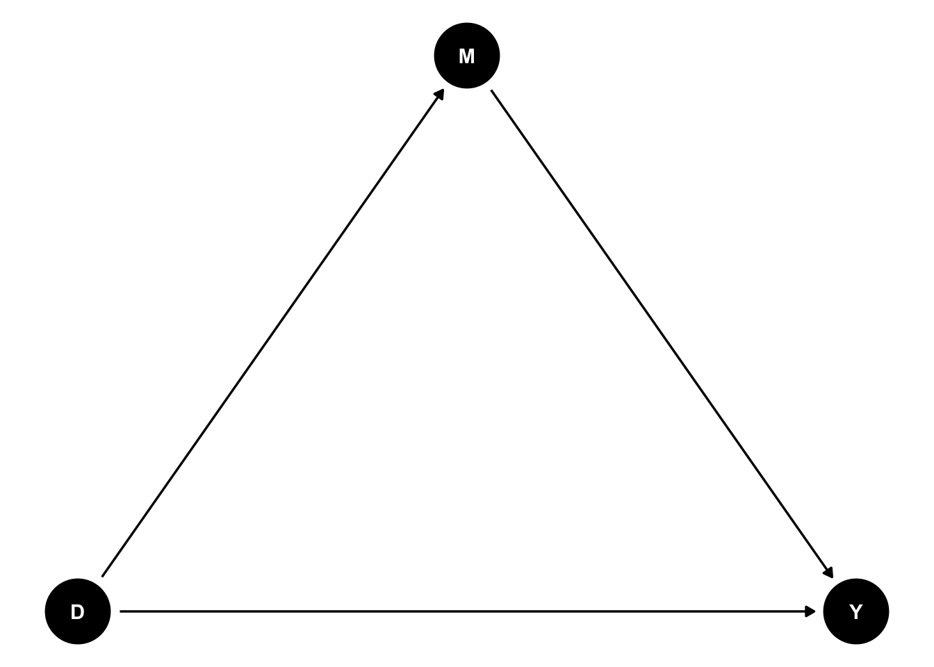
Figure 15.1: DAG of the impact of D on Y partially mediated through M
We are first going to define mediated and unmediated treatment effects and see how they work in our example and we’ll then try to understand better how exactly mediation works and the mechanisms that are behind these treatment effects.
15.1.1 Defining mediated and unmediated treatment effects
Let’s start with a binary mediator, in order to keep things simple: \(M_i\in\left\{0,1\right\}\). We can define four potential outcomes \(Y_i^{d,m}\), \((d,m)\in\left\{0,1\right\}^2\). We can also define two potential outcomes for the mediator: \(M^d_i\), \(d\in\left\{0,1\right\}\).
The switching equation can now be written as follows:
\[\begin{align*} Y_i & = \begin{cases} Y_i^{1,1} & \text{if } D_i=1 \text{ and }M_i=1\\ Y_i^{1,0} & \text{if } D_i=1 \text{ and }M_i=0\\ Y_i^{0,1} & \text{if } D_i=0 \text{ and }M_i=1\\ Y_i^{0,0} & \text{if } D_i=0 \text{ and }M_i=0 \end{cases} \\ & = Y_i^{1,1}D_iM_i + Y_i^{0,1}(1-D_i)M_i + Y_i^{1,0}D_i(1-M_i)+ Y_i^{0,0}(1-D_i)(1-M_i). \end{align*}\]
We are now equipped to define two sets of causal mediation effects: the mediated (or indirect) effect and the unmediated (or direct) effect (we follow Imai, Keene and Tingley (2010)):
\[\begin{align*} \Delta^{Y_{m(d)}}_{i} & = Y_i^{d,M_i^1}-Y_i^{d,M_i^0}\\ \Delta^{Y_{u(d)}}_{i} & = Y_i^{1,M_i^d}-Y_i^{0,M_i^d}. \end{align*}\]
\(\Delta^{Y_{m(d)}}_{i}\) is the causal effect of the treatment on the outcome acting through the mediator only, while keeping the value of the treatment fixed at \(d\). \(\Delta^{Y_{u(d)}}_{i}\) is the causal effect of the treatment on the outcome acting through the treatment only, while keeping the value of the mediator fixed at \(M_i(d)\). In the absence of interaction effects between the treatment and the mediator, we have \(\Delta^{Y_{m(0)}}_{i}=\Delta^{Y_{m(1)}}_{i}=\Delta^{Y_{m}}_{i}\) and \(\Delta^{Y_{u(0)}}_{i}=\Delta^{Y_{u(1)}}_{i}=\Delta^{Y_{u}}_{i}\).
What is nice is that the individual effect of the treatment can be decomposed in these two components:
\[\begin{align*} \Delta^Y_{i} & = Y_i^{1,M_i^1}-Y_i^{0,M_i^0}\\ & = Y_i^{1,M_i^1}-Y_i^{1,M_i^0}+Y_i^{1,M_i^0}-Y_i^{0,M_i^0}=\Delta^{Y_{m(1)}}_{i}+\Delta^{Y_{u(0)}}_{i}\\ & = Y_i^{1,M_i^1}-Y_i^{0,M_i^1}+Y_i^{0,M_i^1}-Y_i^{0,M_i^0}=\Delta^{Y_{u(1)}}_{i}+\Delta^{Y_{m(0)}}_{i}. \end{align*}\]
In the absence of interaction effects between the mediator and the treatment, this decomposition is unique. The decomposition can also be applied to the TT parameter:
\[\begin{align*} \Delta^Y_{TT} & = \esp{Y_i^{1,M_i^1}-Y_i^{0,M_i^0}|D_i=1}\\ & = \Delta^{Y_{m(1)}}_{TT}+\Delta^{Y_{u(0)}}_{TT}\\ & = \Delta^{Y_{u(1)}}_{TT}+\Delta^{Y_{m(0)}}_{TT}, \end{align*}\]
with:
\[\begin{align*} \Delta^{Y_{m(d)}}_{TT} & = \esp{\Delta^{Y_{m(d)}}_{i}|D_i=1}\\ \Delta^{Y_{u(d)}}_{TT} & = \esp{\Delta^{Y_{u(d)}}_{i}|D_i=1}. \end{align*}\]
Here again, the decomposition will be unique if there are no interactions between the treatment and the mediator variable.
Some authors use an alternative definition of the unmediated or direct treatment effect: the controlled direct effect. It is defined as the average effect of the treatment while keeping the mediator at a predefined value:
\[\begin{align*} \Delta^{Y_u(m)}_{TT_c} & = \esp{Y_i^{1,m}-Y_i^{0,m}|D_i=1}. \end{align*}\]
Example 15.1 Let’s see how this works in our example.
The first order of business is to set up a model:
\[\begin{align*} y_i^{1,1} & = y_i^0+\bar{\alpha}+ \tau_1 +\theta\mu_i+\eta_i \\ y_i^{1,0} & = y_i^0+\bar{\alpha}+\theta\mu_i+\eta_i \\ y_i^{0,1} & = \mu_i+\delta + \tau_0+U_i^0 \\ y_i^{0,0} & = \mu_i+\delta+U_i^0 \\ U_i^0 & = \rho U_i^B+\epsilon_i \\ y_i^B & =\mu_i+U_i^B \\ U_i^B & \sim\mathcal{N}(0,\sigma^2_{U}) \\ M_i & = \uns{\xi y_i^B + \psi D_i+ V^M_i\leq\bar{y}_M} \\ V^M_i & = \gamma_M(\mu_i-\bar{\mu}) + \omega^M_i \\ D_i & = \uns{y_i^B+ V_i\leq\bar{y}} \\ V_i & = \gamma(\mu_i-\bar{\mu}) + \omega_i \\ (\eta_i,\omega_i,\omega^M_i) & \sim\mathcal{N}(0,0,0,\sigma^2_{\eta},\sigma^2_{\omega},\sigma^2_{\omega_M},\rho_{\eta,\omega},\rho_{\eta,\omega_M},\rho_{\omega,\omega_M}) \end{align*}\]
Let us choose some parameter values and simulate the model.
param <- c(8,.5,.28,1500,1500,0.9,0.01,0.05,0.05,0.05,0.1,0.2,0.1,1,-0.25,0.1,0.05,7.98,0.28,1,0,0,0)
names(param) <- c("barmu","sigma2mu","sigma2U","barY","barYM","rho","theta","sigma2epsilon","sigma2eta","delta","baralpha","tau1","tau0","xi","psi","gamma","gammaM","baryB","sigma2omega","sigma2omegaM","rhoetaomega","rhoetaomegaM","rhoomegaomegaM")
Let us now simulate the data:
set.seed(1234)
N <-1000
cov.eta.omega.omegaM <- matrix(c(param["sigma2eta"],param["rhoetaomega"]*sqrt(param["sigma2eta"]*param["sigma2omega"]),param["rhoetaomegaM"]*sqrt(param["sigma2eta"]*param["sigma2omegaM"]),
                                 param["rhoetaomega"]*sqrt(param["sigma2eta"]*param["sigma2omega"]),param["sigma2omega"],param["rhoomegaomegaM"]*sqrt(param["sigma2omega"]*param["sigma2omegaM"]),
                                 param["rhoetaomegaM"]*sqrt(param["sigma2eta"]*param["sigma2omegaM"]),param["rhoomegaomegaM"]*sqrt(param["sigma2omega"]*param["sigma2omegaM"]),param["sigma2omegaM"]),ncol=3,nrow=3)
eta.omega <- as.data.frame(mvrnorm(N,c(0,0,0),cov.eta.omega.omegaM))
colnames(eta.omega) <- c('eta','omega','omegaM')
mu <- rnorm(N,param["barmu"],sqrt(param["sigma2mu"]))
UB <- rnorm(N,0,sqrt(param["sigma2U"]))
yB <- mu + UB
YB <- exp(yB)
Ds <- rep(0,N)
V <- param["gamma"]*(mu-param["barmu"])+eta.omega$omega
Ds[yB+V<=log(param["barY"])] <- 1
VM <- param["gammaM"]*(mu-param["barmu"])+eta.omega$omegaM
M <- rep(0,N)
M[param['xi']*yB+param['psi']*Ds+VM<=log(param["barYM"])] <- 1
M1 <- rep(0,N)
M1[param['xi']*yB+param['psi']+VM<=log(param["barYM"])] <- 1
M0 <- rep(0,N)
M0[param['xi']*yB+VM<=log(param["barYM"])] <- 1
epsilon <- rnorm(N,0,sqrt(param["sigma2epsilon"]))
U0 <- param["rho"]*UB + epsilon
alpha <- param["baralpha"]+  param["theta"]*mu + eta.omega$eta
y00 <- mu +  U0 + param["delta"]
y01 <- mu +  U0 + param['tau0']+ param["delta"]
y10 <- y00+alpha
y11 <- y00+alpha+param['tau1']
y1 <- y11*M1+y10*(1-M1)
y0 <- y01*M0+y00*(1-M0)
y1M1 <- y00+alpha+param['tau1']*M1
y1M0 <- y00+alpha+param['tau1']*M0
y0M1 <- y00 + param['tau0']*M1
y0M0 <- y00 + param['tau0']*M0
y <- y11*Ds*M+y10*Ds*(1-M)+y01*(1-Ds)*M+y00*(1-Ds)*(1-M)
Let us finally compute the values of TT and of the mediated and unmediated average treatment effects on the treated in the sample.
# treatment on the treated
TT <- mean(y1[Ds==1]-y0[Ds==1])
# mediated treatment effects
TTm1 <- mean(y1M1[Ds==1]-y1M0[Ds==1])
TTm0 <- mean(y0M1[Ds==1]-y0M0[Ds==1])
# unmediated treatment effects
TTu1 <- mean(y1M1[Ds==1]-y0M1[Ds==1])
TTu0 <- mean(y1M0[Ds==1]-y0M0[Ds==1])

# preparing graph
mediation.example <- data.frame(TT=c(TTm1,TTu0,TTm0,TTu1),Effect=c("TTm1","TTu0","TTm0","TTu1"),Type=c("Mediated","Unmediated","Mediated","Unmediated"),Decomposition=c("m1u0","m1u0","m0u1","m0u1")) %>%
                      mutate(
                        Effect=factor(Effect,levels=c("TTm1","TTu0","TTm0","TTu1")),
                        Type=factor(Type,levels=c("Mediated","Unmediated")),
                        Decomposition=factor(Decomposition,levels=c("m1u0","m0u1"))
                      )
The average effect of the treatment on the treated is equal to 0.243. It can be decomposed in two ways. First, the impact mediated through the mediator \(M_i\) when \(D_i\) is fixed at 1 (0.014) and the effect not mediated through \(M_i\) (with \(M_i\) fixed at \(M_i^0\)) (0.228). Second, the impact mediated through the mediator \(M_i\) when \(D_i\) is fixed at 0 (0.007) and the effect not mediated through \(M_i\) (with \(M_i\) fixed at \(M_i^1\)) (0.235). Let us plot the results:
# plotting the result
ggplot(mediation.example, aes(x=Decomposition, y=TT,fill=Type)) +
  geom_bar(stat="identity")+
  theme_bw()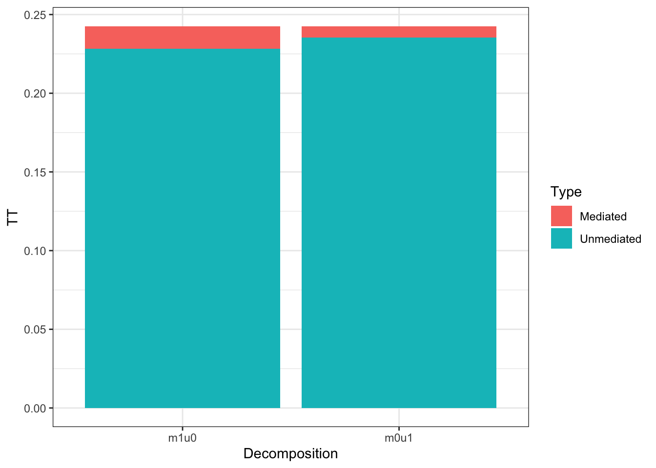
Figure 15.2: Decomposition of the Average Treatment Effect on the Treated in Mediated and Unmediated Effect
As Figure 15.2 shows, most of the effect of the treatment on the outcome is not mediated through \(M_i\) in our example. We can also see that there seems to be limited interaction between the treatment and the mediator since both decompositions yield similar quantities.
15.1.2 Decomposing mediated and unmediated effects
In order to understand better how mediation works, it is very useful to decompose the mediated and unmediated effects using the classical typology of Imbens and Angrist (1994). Let’s define four types by the reactions of their mediators to the treatment:
- Always takers, who always have the mediator set to 1: \(M_i^{1}=M_i^{0}=1\). I denote them \(T_i=a\).
- Never takers, who always have the mediator set to 0: \(M_i^{1}=M_i^{0}=0\). I denote them \(T_i=n\).
- Compliers, whose value of the mediator moves from 0 to 1 when the value of the treatment variable changes from 0 to 1: \(M_i^{1}=1\) and \(M_i^{0}=0\). I denote them \(T_i=c\).
- Defiers, whose value of the mediator switches from 1 to 0 when the value of the treatment variable changes from 0 to 1: \(M_i^{1}=0\) and \(M_i^{0}=1\). I denote them \(T_i=d\).
\(T_i\) spans all the potential reactions of the mediator to the treatment, and thus \(\cup_{t\in\{a,n,c,d\}}\{T_i=t\}\) is a partition of the sampling space. It is very interesting to decompose both the full treatment effect on the treated but also the mediated and unmediated treatment effects on the treated in terms of the \(T_i\) variable. Let’s go. The Treatment on the Treated parameter first:
\[\begin{align*} \Delta^Y_{TT} & = \esp{Y_i^{1,M_i^1}-Y_i^{0,M_i^0}|D_i=1}\\ & = \sum_{t\in\{a,n,c,d\}}\esp{Y_i^{1,M_i^1}-Y_i^{0,M_i^0}|T_i=t,D_i=1}\Pr(T_i=t|D_i=1)\\ & = \esp{Y_i^{1,1}-Y_i^{0,1}|T_i=a,D_i=1}\Pr(T_i=a|D_i=1)\\ & \phantom{=}+\esp{Y_i^{1,0}-Y_i^{0,0}|T_i=n,D_i=1}\Pr(T_i=n|D_i=1)\\ & \phantom{=}+\esp{Y_i^{1,1}-Y_i^{0,0}|T_i=c,D_i=1}\Pr(T_i=c|D_i=1)\\ & \phantom{=}+\esp{Y_i^{1,0}-Y_i^{0,1}|T_i=d,D_i=1}\Pr(T_i=d|D_i=1). \end{align*}\]
Let us now look at the average mediated effect on the treated:
\[\begin{align*} \Delta^{Y_{m(1)}}_{TT} & = \esp{Y_i^{1,M_i^1}-Y_i^{1,M_i^0}|D_i=1}\\ & = \sum_{t\in\{a,n,c,d\}}\esp{Y_i^{1,M_i^1}-Y_i^{1,M_i^0}|T_i=t,D_i=1}\Pr(T_i=t|D_i=1)\\ & = \esp{Y_i^{1,1}-Y_i^{1,1}|T_i=a,D_i=1}\Pr(T_i=a|D_i=1)\\ & \phantom{=}+\esp{Y_i^{1,0}-Y_i^{1,0}|T_i=n,D_i=1}\Pr(T_i=n|D_i=1)\\ & \phantom{=}+\esp{Y_i^{1,1}-Y_i^{1,0}|T_i=c,D_i=1}\Pr(T_i=c|D_i=1)\\ & \phantom{=}+\esp{Y_i^{1,0}-Y_i^{1,1}|T_i=d,D_i=1}\Pr(T_i=d|D_i=1)\\ & = \esp{Y_i^{1,1}-Y_i^{1,0}|T_i=c,D_i=1}\Pr(T_i=c|D_i=1)\\ & \phantom{=}-\esp{Y_i^{1,1}-Y_i^{1,0}|T_i=d,D_i=1}\Pr(T_i=d|D_i=1). \end{align*}\]
The result above is very useful and provides several fruitful insights. First, the average mediated effect on the treated only involves the effects on the compliers and the defiers. That is, only units whose value of the mediator is affected by the treatment are part of the mediated treatment effect. Second, their importance in the mediated treatment effect depends on their proportion in the (treated) population. That is, if few units have their value of the mediator affected by the treatment, the size of the mediated treatment effect decreases. Finally, the impact of the mediator on the defiers enters with a negative weight in the definition of the mediated treatment effect. This makes sense, since the treatment makes these units experience lower values of the mediator.
Finally, let us decompose the unmediated treatment effect on the treated:
\[\begin{align*} \Delta^{Y_{u(0)}}_{TT} & = \esp{Y_i^{1,M_i^0}-Y_i^{0,M_i^0}|D_i=1}\\ & = \sum_{t\in\{a,n,c,d\}}\esp{Y_i^{1,M_i^0}-Y_i^{0,M_i^0}|T_i=t,D_i=1}\Pr(T_i=t|D_i=1)\\ & = \esp{Y_i^{1,1}-Y_i^{0,1}|T_i=a,D_i=1}\Pr(T_i=a|D_i=1)\\ & \phantom{=}+\esp{Y_i^{1,0}-Y_i^{0,0}|T_i=n,D_i=1}\Pr(T_i=n|D_i=1)\\ & \phantom{=}+\esp{Y_i^{1,0}-Y_i^{0,0}|T_i=c,D_i=1}\Pr(T_i=c|D_i=1)\\ & \phantom{=}+\esp{Y_i^{1,1}-Y_i^{0,1}|T_i=d,D_i=1}\Pr(T_i=d|D_i=1). \end{align*}\]
The unmediated treatment effect on the treated is equal to the direct effect of the treatment on each of the types multiplied by their proportion in the (treated) population, keeping the value of the mediator at its default value when the treatment is equal to 0.
15.2 The Fundamental Problem of Mediation Analysis
In this section, we state the Fundamental Problem of Mediation Analysis (FPMA) and we then move on to examining the biases of intuitive comparisons that could be used to recover the mediated and unmediated effects of the treatment.
15.2.1 The Fundamental Problem of Mediation Analysis
Mediation analysis is hard. It is even harder than identification and estimation of treatment effects. The following theorem shows formally why this is the case:
Theorem 15.1 (Fundamental Problem of Mediation Analysis) The mediated and unmediated treatment effects are fundamentally unobservable.
Proof. Let’s look at the mediated treatment effect first. It can be decomposed as follows:
\[\begin{align*} \Delta^{Y_{m(1)}}_{TT} & = \esp{Y_i^{1,M_i^1}-Y_i^{1,M_i^0}|D_i=1}\\ & = \esp{Y_i^{1,M_i^1}-Y_i^{1,M_i^0}|D_i=1,M_i=1}\Pr(M_i=1|D_i=1)\\ & \phantom{=} + \esp{Y_i^{1,M_i^1}-Y_i^{1,M_i^0}|D_i=1,M_i=0}\Pr(M_i=0|D_i=1)\\ & = \esp{Y^{1,1}_i-Y_i^{1,M_i^0}|D_i=1,M_i=1}\Pr(M_i=1|D_i=1)\\ & \phantom{=} + \esp{Y^{1,0}_i-Y_i^{1,M_i^0}|D_i=1,M_i=0}\Pr(M_i=0|D_i=1)\\ & = (\esp{Y_i|D_i=1,M_i=1}-\esp{Y_i^{1,M_i^0}|D_i=1,M_i=1})\Pr(M_i=1|D_i=1)\\ & \phantom{=} + (\esp{Y_i|D_i=1,M_i=0}-\esp{Y_i^{1,M_i^0}|D_i=1,M_i=0})\Pr(M_i=0|D_i=1), \end{align*}\]
where the second and third inequalities follow from the switching equation. Note that both \(\esp{Y_i^{1,M_i^0}|D_i=1,M_i=1}\) and \(\esp{Y_i^{1,M_i^0}|D_i=1,M_i=0}\) are counterfactual values that cannot be observed (they depend on the value of the mediator when \(D_i=0\), which is unobserved when \(D_i=1\)).
Let us look at the unmediated treatment effect now:
\[\begin{align*} \Delta^{Y_{u(1)}}_{TT} & = \esp{Y_i^{1,M_i^1}-Y_i^{0,M_i^1}|D_i=1}\\ & = \esp{Y_i^{1,M_i^1}-Y_i^{0,M_i^1}|D_i=1,M_i=1}\Pr(M_i=1|D_i=1)\\ & \phantom{=} + \esp{Y_i^{1,M_i^1}-Y_i^{0,M_i^1}|D_i=1,M_i=0}\Pr(M_i=0|D_i=1)\\ & = \esp{Y^{1,1}_i-Y_i^{0,M_i^1}|D_i=1,M_i=1}\Pr(M_i=1|D_i=1)\\ & \phantom{=} + \esp{Y^{1,0}_i-Y_i^{0,M_i^1}|D_i=1,M_i=0}\Pr(M_i=0|D_i=1)\\ & = (\esp{Y_i|D_i=1,M_i=1}-\esp{Y_i^{0,M_i^1}|D_i=1,M_i=1})\Pr(M_i=1|D_i=1)\\ & \phantom{=} + (\esp{Y_i|D_i=1,M_i=0}-\esp{Y_i^{0,M_i^1}|D_i=1,M_i=0})\Pr(M_i=0|D_i=1), \end{align*}\]
Note that both \(\esp{Y_i^{0,M_i^1}|D_i=1,M_i=1}\) and \(\esp{Y_i^{0,M_i^1}|D_i=1,M_i=0}\) are counterfactual values that cannot be observed (they depend on the value of the outcome when \(D_i=0\), which is unobserved when \(D_i=1\)).
Remark. The key to understanding Theorem 15.1 is to see that the potential value of the mediator is unknown and this combines with the fact that the potential value of the outcome had the mediator or the treatment changed value is also unobserved.
15.2.2 Biases of Intuitive Comparisons
Usual intuitive proxies for the mediated and unmediated effects are usually biased because of confounders. We can visualize the problem in a DAG, with the arcs indicating the existence of confounders between two variables:
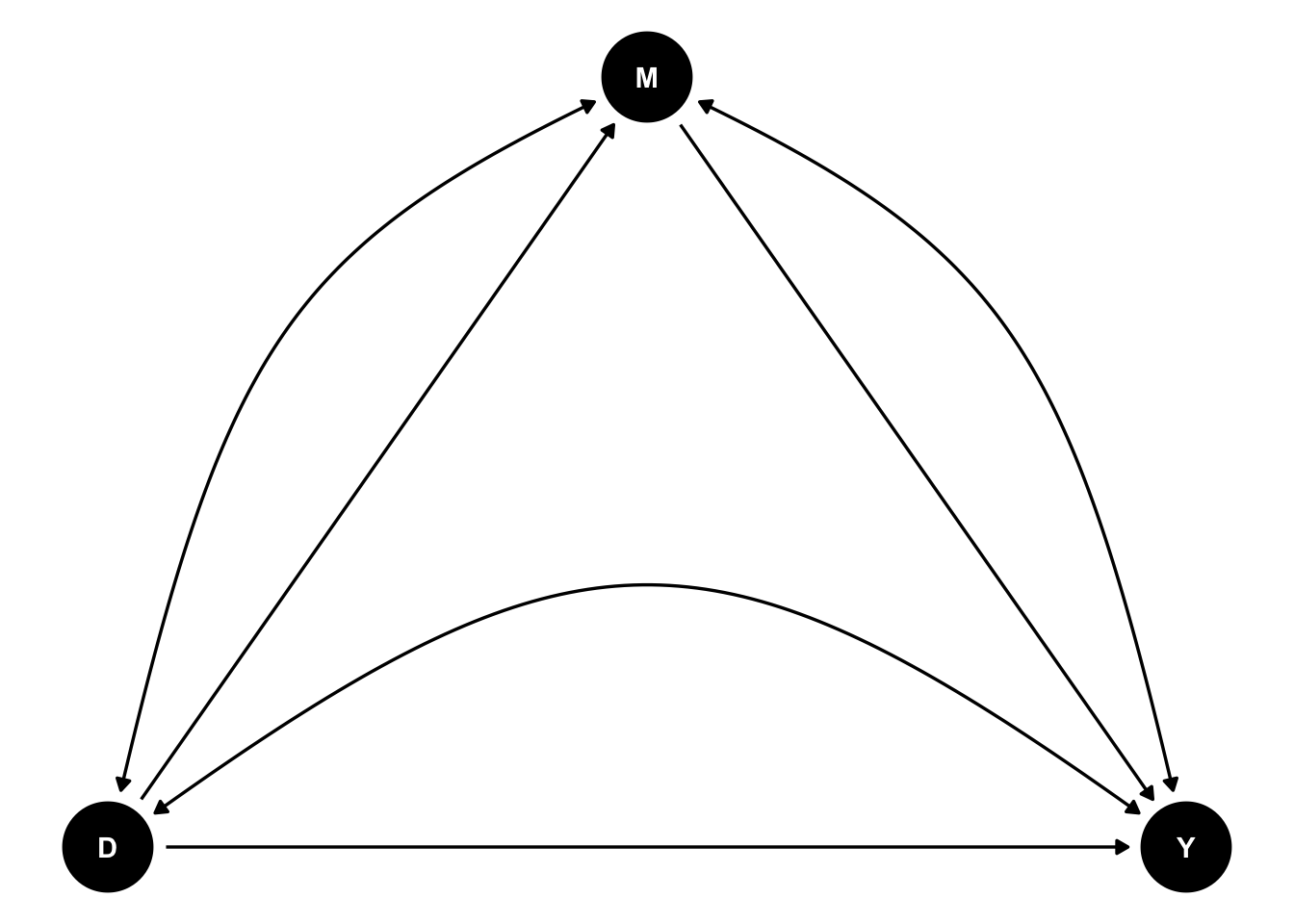
Figure 15.3: DAG of a confounded mediating relationship
The most obvious intuitive comparison that could try to recover mediated and unmediated treatment effects is the conditional With/Without comparison:
\[\begin{align*} \Delta^Y_{WW|D_i=d} & = \esp{Y_i|D_i=d,M_i=1}-\esp{Y_i|D_i=d,M_i=0}\\ \Delta^Y_{WW|M_i=m} & = \esp{Y_i|D_i=1,M_i=m}-\esp{Y_i|D_i=0,M_i=m}. \end{align*}\]
Our hope is that \(\Delta^Y_{WW|D_i=d}\) recovers the mediated treatment effect and \(\Delta^Y_{WW|M_i=d}\) recovers the unmediated treatment effect. Unfortunately, that is not generally the case. The following theorem makes this point clear:
Theorem 15.2 (Bias of the Conditional With/Without Comparisons) The conditional With/Without comparisons are biased estimators of the mediated and unmediated average effects of the treatment on the treated:
\[\begin{align*} \Delta^Y_{WW|D_i=1} & = \Delta^{Y_{m(1)}}_{TT|M_i=1}+\Delta^{Y^{1,0}}_{SB^{m(1)}|D_i=1}\\ \Delta^Y_{WW|M_i=1} & = \Delta^{Y_{u(1)}}_{TT|M_i=1}+\Delta^{Y^{0,1}}_{SB^{u(1)}|M_i=1}. \end{align*}\]
with
\[\begin{align*} \Delta^{Y_{m(1)}}_{TT|M_i=1} & = \esp{Y_i^{1,1}-Y_i^{1,0}|D_i=1,M_i=1}\\ \Delta^{Y^{1,0}}_{SB^{m(1)}|D_i=1} & = \esp{Y^{1,0}_i|D_i=1,M_i=1}-\esp{Y^{1,0}_i|D_i=1,M_i=0}\\ \Delta^{Y_{u(1)}}_{TT|M_i=1} & = \esp{Y_i^{1,1}-Y_i^{0,1}|D_i=1,M_i=1}\\ \Delta^{Y^{0,1}}_{SB^{u(1)}|M_i=1} & = \esp{Y^{0,1}_i|D_i=1,M_i=1}-\esp{Y^{0,1}_i|D_i=0,M_i=0}. \end{align*}\]
Proof. The proof is straightforward using the switching equation and adding and subtracting the counterfactual part of the treatment effects.
According to Theorem 15.2, Selection Bias biases the conditional With/Without estimators of the mediated and unmediated treatment effects. As Figure @(ref:DAGMediationConfounded) suggests, this is because confounders are correlated with both treatment, mediator and outcome. The most important confounder in our example is \(\mu_i\), which is correlated with all three variables.
Remark. Note that Theorem 15.2 shows the bias for the mediated and unmediated treatment effects conditional on \(M_i=1\). The same results with the unconditional version of the treatment effects would be somewhat more intricate since it would involve weights.
Remark. Note also that Theorem 15.2 shows the bias for the mediated and unmediated treatment effects with \(m(1)\) and \(u(1)\) as indices. The same results with \(m(0)\) and \(u(0)\) are similar.
Example 15.2 Let’s see how that works our in our example.
# mediated treatment effect for M=1
TTm1M1 <- mean(y11[Ds==1&M==1])-mean(y10[Ds==1&M==1])
# unmediated treatment effect for M==1
TTu1M1 <- mean(y11[Ds==1&M==1])-mean(y01[Ds==1&M==1])

# selection bias for the mediated treatment effect
SBm1D1 <- mean(y10[Ds==1&M==1])-mean(y10[Ds==1&M==0])
# selection bias for the unmediated treatment effect
SBu1M1 <- mean(y01[Ds==1&M==1])-mean(y01[Ds==0&M==1])

# with/without comparison for the mediated treatment effect for M=1
WWD1 <- mean(y[Ds==1&M==1])-mean(y[Ds==1&M==0])
# unmediated treatment effect for M==1
WWM1 <- mean(y[Ds==1&M==1])-mean(y[Ds==0&M==1])
In our example, the With/Without estimator of the mediated treatment effect is equal to -0.239 (for \(D_i=1\)). The true mediated treatment effect for \(D_i=1\) and \(M_i=1\) is equal to 0.2. Selection bias for the mediated treatment effect for \(D_i=1\) is thus equal to -0.439. The With/Without estimator of the unmediated treatment effect is equal to -0.571 (for \(M_i=1\)). The true unmediated treatment effect for \(D_i=1\) and \(M_i=1\) is equal to 0.253. Selection bias for the unmediated treatment effect for \(M_i=1\) is thus equal to -0.824.
15.3 Mediation analysis with experimental data
Imai, Tingleu and Yamamoto (2013) propose two experimental designs to recover the mediated and unmediated treatment effects: the parallel design and the crossover design. We are going to also study identification in a Sequential Self-Selection design, which I find slightly simpler. Let’s examine these approaches in turn.
15.3.1 Mediation analysis in the Parallel design
In the parallel design, we run a three-step experiment. In the first step, we randomly allocate units either to the first or the second arm of the experiment. We denote \(R^1_i=0\) the first arm and \(R^1_i=1\) the second arm.
In the first arm, we randomly allocate the treatment among units and we let the mediator take the corresponding value without interferring. We denote \(R^2_i=1\) when unit \(i\) is assigned to the treatment and \(R^2_i=0\) when unit \(i\) us not assigned to the treatment. In this design, we assume that units fully comply with the assignment. One way to do that is to run the whole parallel design only on units that are selected into the treatment (\(D_i=1\)).
In the second arm, we run a two-step experiment. In the first step, we randomly allocate units either to the treatment or to the control. We denote \(R_i^2=1\) when unit \(i\) is assigned to the treatment and \(R_i^2=0\) when it is assigned to the control. In the second step, we randomly allocate units to the mediator. We denote \(R_i^3=1\) when unit \(i\) is assigned to the mediator value \(M_i=1\) and \(R_i^3=0\) when unit \(i\) is assigned to the mediator value of \(M_i=0\).
In order to recover the treatment effect on the treated, we are going to assume that the experiment takes place among the units selected to participate in the treatment, i.e. among units with \(D_i=1\). If we abstract from this, the parameter we recover is the average effect of the treatment, ATE.
Let us formalize the assumptions we make on the Parallel design
Hypothesis 15.1 (Sequential Independence in the Parallel Design) We assume that the sequential randomized allocation of the program among applicants is well done:
\[\begin{align*} R^1_i & \Ind(Y_i^{00},Y_i^{01},Y_i^{10},Y_i^{11},M^1_i,M^0_i)|D_i=1\\ R^2_i & \Ind(Y_i^{00},Y_i^{01},Y_i^{10},Y_i^{11},M^1_i,M^0_i)|R_i^1,D_i=1\\ R^3_i & \Ind(Y_i^{00},Y_i^{01},Y_i^{10},Y_i^{11},M^1_i,M^0_i)|R_i^2,R_i^1=1,D_i=1. \end{align*}\]
We need a second assumption:
Hypothesis 15.2 (Validity of the Sequential Parallel Design) We assume that the sequential randomized allocation of the program does not interfere with how potential outcomes and potential treatment and mediator choices are generated:
\[\begin{align*} Y_i & = \begin{cases} Y_i^{11} & \text{ if } D_i=1 \text{ and } ((R^1_i=0 \text{ and } R^2_i=1 \text{ and } M_i=1) \text{ or } (R^1_i=1 \text{ and } R^2_i=1 \text{ and } R^3_i=1)) \\ Y_i^{10} & \text{ if } D_i=1 \text{ and } ((R^1_i=0 \text{ and } R^2_i=1 \text{ and } M_i=0) \text{ or } (R^1_i=1 \text{ and } R^2_i=1 \text{ and } R^3_i=0)) \\ Y_i^{01} & \text{ if } D_i=1 \text{ and } ((R^1_i=0 \text{ and } R^2_i=0 \text{ and } M_i=1) \text{ or } (R^1_i=1 \text{ and } R^2_i=0 \text{ and } R^3_i=1)) \\ Y_i^{00} & \text{ if } D_i=1 \text{ and } ((R^1_i=0 \text{ and } R^2_i=0 \text{ and } M_i=0) \text{ or } (R^1_i=1 \text{ and } R^2_i=0 \text{ and } R^3_i=0)) \\ \end{cases}\\ M_i & = \begin{cases} M_i^{1} & \text{ if } D_i=1 \text{ and }R^1_i=0\text{ and } R^2_i=1\\ M_i^{0} & \text{ if } D_i=1 \text{ and }R^1_i=0\text{ and } R^2_i=0 \end{cases}, \end{align*}\]
with \((Y_i^{00},Y_i^{01},Y_i^{10},Y_i^{11},M^1_i,M^0_i)\) the same potential outcomes and potential treatment and mediator choices as in a routine allocation of the treatment.
Remark. Assumption 15.2 imposes that the experimental setting does not alter the treatment, mediator and outcomes of the agents.
For identification of the mediated and unmediated effects to go through, we need a final (strong) assumption: the absence of interaction effects:
Hypothesis 15.3 (Absence of Interaction Effects) We assume that the treatment and the mediator do not interact: \(Y_i^{d,m}-Y_i^{d,m'}=Y_i^{d',m}-Y_i^{d',m'}\), \(\forall (d,m,d'm')\in\{0,1\}^4\), \(d\neq d'\), \(m\neq m'\).
Remark. Assumption 15.3 is actually too strong for our result. We only need that the assumption holds for the average effects on the never takers, defiers and compliers.
Remark. Under Assumption 15.3, \(\Delta^{Y_{u(1)}}_{TT}=\Delta^{Y_{u(0)}}_{TT}\), which we denote \(\Delta^{Y_{u(d)}}_{TT}\) and \(\Delta^{Y_{m(1)}}_{TT}=\Delta^{Y_{m(0)}}_{TT}\), which we denote \(\Delta^{Y_{m(d)}}_{TT}\).
Under these assumptions, we have the following result:
Theorem 15.3 (Identification of Total, Mediated and Unmediated Effects in the Parallel Design) Under Assumptions 15.1, 15.2 and 15.3, the treatment effect on the treated and the mediated and unmediated effects on the treated are identified in the Parallel Design:
\[\begin{align*} \Delta^Y_{TT} & = \esp{Y_i|D_i=1,R^1_i=0,R_i^2=1}-\esp{Y_i|D_i=1,R^1_i=0,R_i^2=0}\\ \Delta^{Y_{u(d)}}_{TT} & = \esp{Y_i|D_i=1,R^1_i=1,R_i^2=1,R_i^3=1}-\esp{Y_i|D_i=1,R^1_i=1,R_i^2=0,R_i^3=1}\\ & =\esp{Y_i|D_i=1,R^1_i=1,R_i^2=1,R_i^3=0}-\esp{Y_i|D_i=1,R^1_i=1,R_i^2=0,R_i^3=0}\\ \Delta^{Y_{m(d)}}_{TT} & = \esp{Y_i|D_i=1,R^1_i=0,R_i^2=1}-\esp{Y_i|D_i=1,R^1_i=0,R_i^2=0}\\ & \phantom{=}-\esp{Y_i|D_i=1,R^1_i=1,R_i^2=1,R_i^3=1}-\esp{Y_i|D_i=1,R^1_i=1,R_i^2=0,R_i^3=1}\\ & = \esp{Y_i|D_i=1,R^1_i=0,R_i^2=1}-\esp{Y_i|D_i=1,R^1_i=0,R_i^2=0}\\ & \phantom{=}-\esp{Y_i|D_i=1,R^1_i=1,R_i^2=1,R_i^3=0}-\esp{Y_i|D_i=1,R^1_i=1,R_i^2=0,R_i^3=0}. \end{align*}\]
Proof. I omit conditioning on \(D_i=1\) to save notation. Let us start with the total effect: \(\esp{Y_i|R^1_i=0,R_i^2=1}-\esp{Y_i|R^1_i=0,R_i^2=0}\) is a With/Without estimator where the treatment has been randomized among a random sample of the units selected to receive the treatment. Theorem 3.2 proves that it identifies \(\Delta^Y_{TT}\) under Assumptions 15.1 and 15.2. The unmediated treatment effect can be recovered as follows:
\[\begin{align*} \esp{Y_i|R^1_i=1,R_i^2=1,R_i^3=1} & -\esp{Y_i|R^1_i=1,R_i^2=0,R_i^3=1} \\ & = \sum_{t\in\{a,n,c,d\}}\esp{Y_i^{1,1}-Y_i^{0,1}|T_i=t}\Pr(T_i=t)\\ \esp{Y_i|R^1_i=1,R_i^2=1,R_i^3=0} & -\esp{Y_i|R^1_i=1,R_i^2=0,R_i^3=0} \\ & = \sum_{t\in\{a,n,c,d\}}\esp{Y_i^{1,0}-Y_i^{0,0}|T_i=t}\Pr(T_i=t), \end{align*}\]
using Assumptions 15.1 and 15.2. Using the decomposition of \(\Delta^Y_{TT}\) in the effects on each type, we have:
\[\begin{align*} \esp{Y_i|R^1_i=0,R_i^2=1} & -\esp{Y_i|R^1_i=0,R_i^2=0}\\ & - (\esp{Y_i|R^1_i=1,R_i^2=1,R_i^3=1} -\esp{Y_i|R^1_i=1,R_i^2=0,R_i^3=1}) \\ & = \esp{Y_i^{0,1}-Y_i^{0,0}|T_i=c}\Pr(T_i=c) \\ & \phantom{=}-\esp{Y_i^{1,1}-Y_i^{1,0}|T_i=d}\Pr(T_i=d)\\ & \phantom{=}+(\esp{Y_i^{1,0}-Y_i^{0,0}|T_i=n}-\esp{Y_i^{1,1}-Y_i^{0,1}|T_i=n})\Pr(T_i=n). \end{align*}\]
and
\[\begin{align*} \esp{Y_i|R^1_i=0,R_i^2=1} & -\esp{Y_i|R^1_i=0,R_i^2=0}\\ & - (\esp{Y_i|R^1_i=1,R_i^2=1,R_i^3=0} -\esp{Y_i|R^1_i=1,R_i^2=0,R_i^3=0}) \\ & = \esp{Y_i^{1,1}-Y_i^{1,0}|T_i=c}\Pr(T_i=c) \\ & \phantom{=}-\esp{Y_i^{0,1}-Y_i^{0,0}|T_i=d}\Pr(T_i=d)\\ & \phantom{=}+(\esp{Y_i^{1,1}-Y_i^{0,1}|T_i=a}-\esp{Y_i^{1,0}-Y_i^{0,0}|T_i=a})\Pr(T_i=a). \end{align*}\]
Using Assumption 15.3 and the decomposition formulae for the mediated and unmediated treatment effects on the treated gives the result.
Remark. The proof of Theorem 15.3 is more detailed and explanatory than the one in Imai, Tingleu and Yamamoto (2013). We understand why we need Assumption 15.3: the effects on the always takers and on the never takers estimated in the two treatment arms do not cancel out and the effects of the mediator on the compliers and defiers are not the correct combination in both comparisons unless we make Assumption 15.3.
Remark. Note that the model is overidentified under Assumptions 15.1, 15.2 and 15.3. There are two different ways to estimate the unmediated treatment effect and thus one can test Assumption 15.3 by comparing these two estimates.
Remark. Since the model is overidentified under Assumptions 15.1, 15.2 and 15.3, one wonders what can exactly be identified on the mediated and unmediated treatment effects under these assumptions. Maybe it is possible to bound the treatment effects. This is, to my knowledge, still an open question.
Remark. Imai, Tingleu and Yamamoto (2013) also discuss a Parallel Encouragement design where units are not forced to take the assigned value of the mediator but can be randomly encouraged to do so. They derive sharp bounds on the mediated effect on the compliers in that design.
15.3.2 Mediation analysis in the Sequential Self-Selection design
In a Sequential Self-Selection design, researchers run a Randomized Controlled Trial (RCT) in two-steps. In the first step, the treatment is randomized among those who applied for it. In the second step, the mediator is randomized among those who applied for it. We thus have two random variables \(R_i^1\) and \(R_i^2\) which take values zero or one for observations for which \(D_i=1\) for the first and \(D_i=1\) and \(M_i=1\) for the second.
Let us formalize how the Sequential Self-Selection design works.
Hypothesis 15.4 (Sequential Independence Among Self-Selected) We assume that the sequential randomized allocation of the program among applicants is well done:
\[\begin{align*} R^1_i & \Ind(Y_i^{00},Y_i^{01},Y_i^{10},Y_i^{11},M^1_i,M^0_i)|D_i=1\\ R^2_i & \Ind(Y_i^{00},Y_i^{01},Y_i^{10},Y_i^{11},M^1_i,M^0_i)|R^1_i,M_i=1,D_i=1 \end{align*}\]
We need a second assumption:
Hypothesis 15.5 (Validity of the Sequential Self-Selection design) We assume that the sequential randomized allocation of the program does not interfere with how potential outcomes and self-selection are generated:
\[\begin{align*} Y_i & = \begin{cases} Y_i^{11} & \text{ if } (D_i=1 \text{ and } R^1_i=1 \text{ and } M_i=1 \text{ and } R^2_i=1) \\ Y_i^{10} & \text{ if } ((D_i=1 \text{ and } R^1_i=1) \text{ and } ((M_i=1 \text{ and } R^2_i=0) \text{ or } M_i=0)) \\ Y_i^{01} & \text{ if } (D_i=1 \text{ and } R^1_i=0 \text{ and } M_i=1 \text{ and } R^2_i=1) \\ Y_i^{00} & \text{ if } ((D_i=1 \text{ and } R^1_i=0) \text{ and } ((M_i=1 \text{ and } R^2_i=0) \text{ or } M_i=0)) \end{cases}\\ M_i & = \begin{cases} M_i^{1} & \text{ if } D_i=1 \text{ and } R^1_i=1\\ M_i^{0} & \text{ if } D_i=1 \text{ and } R^1_i=0 \end{cases} \end{align*}\]
with \((Y_i^{00},Y_i^{01},Y_i^{10},Y_i^{11},M^1_i,M^0_i)\) the same potential outcomes and self-selection decisions as in a routine allocation of the treatment.
We finally need a monotonicity assumption:
Hypothesis 15.6 (Monotonicity of the Effect of the Treatment on the Mediator) We assume that the effect of the treatment on the mediator is monotonous:
\[\begin{align*} \Pr(M_i^1-M_i^0<0) & =0. \end{align*}\]
Remark. Assumption 15.6 is equivalent to the absence of defiers: \(\Pr(T_i=d)=0\).
Under these assumptions, we have the following result:
Theorem 15.4 (Identification of Total, Mediated and Unmediated Effects in a Sequential Self-Selection design) Under Assumptions 15.4, 15.5 and 15.6, the treatment effect on the treated and the mediated and unmediated effects are identified in a Sequential Self-Selection Design:
\[\begin{align*} \Delta^Y_{TT} & = \esp{Y_i|D_i=1,R_i^1=1,M_i=1,R_i^2=1}\Pr(M_i=1|D_i=1,R_i^1=1)\\ & \phantom{=}+\esp{Y_i|D_i=1,R_i^1=1,M_i=0}\Pr(M_i=0|D_i=1,R_i^1=1)\\ & \phantom{=}-\left(\esp{Y_i|D_i=1,R_i^1=0,M_i=1,R_i^2=1}\Pr(M_i=1|D_i=1,R_i^1=0)\right.\\ & \phantom{=-(}\left.+\esp{Y_i|D_i=1,R_i^1=0,M_i=0}\Pr(M_i=0|D_i=1,R_i^1=0)\right)\\ \Delta^{Y_{m(1)}}_{TT} & =\left(\esp{Y_i|D_i=1,R_i^1=1,M_i=1,R_i^2=1}\right.\\ &\phantom{=-(}\left.-\esp{Y_i|D_i=1,R_i^1=1,M_i=1,R_i^2=0}\right)\Pr(M_i=1|D_i=1,R_i^1=1)\\ & \phantom{=}-\left(\esp{Y_i|D_i=1,R_i^1=0,M_i=1,R_i^2=1}\right.\\ &\phantom{=-(}\left.-\esp{Y_i|D_i=1,R_i^1=0,M_i=1,R_i^2=0}\right)\Pr(M_i=1|D_i=1,R_i^1=0)\\ \Delta^{Y_{u(0)}}_{TT} & =\Delta^Y_{TT}-\Delta^{Y_{m(1)}}_{TT}. \end{align*}\]
Proof. I omit conditioning on \(D_i=1\) all along to save on notation. Note that:
\[\begin{align*} \esp{Y_i|R_i^1=1,M_i=1,R_i^2=1} & = \esp{Y^{1,M_i^1}_i|R_i^1=1,M^1_i=1,R_i^2=1}\\ & = \esp{Y^{1,M_i^1}_i|M^1_i=1}\\ \esp{Y_i|R_i^1=1,M_i=0} & = \esp{Y^{1,M_i^1}_i|M^1_i=0}\\ \esp{Y_i|R_i^1=0,M_i=1,R_i^2=1} & = \esp{Y^{0,M_i^0}_i|M^0_i=1}\\ \esp{Y_i|R_i^1=0,M_i=0} & = \esp{Y^{0,M_i^0}_i|M^0_i=0}\\ \Pr(M_i=1|R_i^1=1) & = \Pr(M^1_i=1)\\ \Pr(M_i=0|R_i^1=1) & = \Pr(M^1_i=0)\\ \Pr(M_i=1|R_i^1=0) & = \Pr(M^0_i=1)\\ \Pr(M_i=0|R_i^1=0) & = \Pr(M^0_i=0), \end{align*}\]
using Assumptions 15.4 and 15.5. Because \(M_i^1\) and \(M_i^0\) are both partitions of the sampling space, we can use the Law of Iterated Expectations to find:
\[\begin{align*} \esp{Y^{1,M_i^1}_i} &= \esp{Y^{1,M_i^1}_i|M^1_i=1}\Pr(M^1_i=1)+\esp{Y^{1,M_i^1}_i|M^1_i=1}\Pr(M^1_i=0)\\ \esp{Y^{0,M_i^0}_i} &= \esp{Y^{0,M_i^0}_i|M^0_i=1}\Pr(M^0_i=1)+\esp{Y^{0,M_i^0}_i|M^1_i=1}\Pr(M^0_i=0) \end{align*}\]
The difference between the two terms is the definition of \(\Delta^Y_{TT}\). This proves the first part of the theorem.
Note that, under Assumptions 15.4, 15.5 and especially 15.6:
\[\begin{align*} \esp{Y_i|R_i^1=1,M_i=1,R_i^2=1} & -\esp{Y_i|R_i^1=1,M_i=1,R_i^2=0}\\ & = \esp{Y^{11}_i|M^1_i=1} -\esp{Y^{10}_i|M^1_i=1}\\ & = \esp{Y^{11}_i|T_i=a}\Pr(T_i=a|M_i^1=1)+\esp{Y^{11}_i|T_i=c}\Pr(T_i=c|M_i^1=1)\\ & \phantom{=}-\esp{Y^{10}_i|T_i=a}\Pr(T_i=a|M^1_i=1)-\esp{Y^{10}_i|T_i=c}\Pr(T_i=c|M^1_i=1)\\ & = \esp{Y^{11}_i-Y^{10}_i|T_i=a}\Pr(T_i=a|M_i^1=1)\\ & \phantom{=}+\esp{Y^{11}_i-Y^{10}_i|T_i=c}\Pr(T_i=c|M_i^1=1). \end{align*}\]
By the same reasoning, we also have:
\[\begin{align*} \esp{Y_i|R_i^1=0,M_i=1,R_i^2=1} & -\esp{Y_i|R_i^1=0,M_i=1,R_i^2=0}\\ & = \esp{Y^{11}_i|M^0_i=1} -\esp{Y^{10}_i|M^0_i=1}\\ & = \esp{Y^{11}_i-Y^{10}_i|T_i=a}. \end{align*}\]
Finally, using Bayes Law and the fact that:
\[\begin{align*} \Pr(M_i=1|R_i^1=1) & = \Pr(M^1_i=1) = \Pr(T_i=a)+\Pr(T_i=c)\\ \Pr(M_i=1|R_i^1=0) & = \Pr(M^0_i=1) = \Pr(T_i=a), \end{align*}\]
we have that \(\Pr(T_i=a|M_i^1=1)=\frac{\Pr(T_i=a)}{\Pr(T_i=a)+\Pr(T_i=c)}\) and \(\Pr(T_i=c|M_i^1=1)=\frac{\Pr(T_i=c)}{\Pr(T_i=a)+\Pr(T_i=c)}\). Combining the results with the decomposition of \(\Delta^{Y_{m(1)}}_{TT}\) under Assumption 15.6 proves the identification of \(\Delta^{Y_{m(1)}}_{TT}\). The identification of \(\Delta^{Y_{u(0)}}_{TT}\) comes directly from the decompositions of \(\Delta^Y_{TT}\), \(\Delta^{Y_{m(1)}}_{TT}\) and \(\Delta^{Y_{u(0)}}_{TT}\) under Assumption 15.6. This proves the result.
Remark. Intuitively, Theorem 15.4 works by using what happens in the voluntary parts of both experimental arms (the parts where the mediator value chosen by the units is given to them) to recover the treatment effect on the treated. Then, the With/Without estimators using \(R_i^2\) in each arm give the effect of the mediator, on the always treated and the compliers in the arm where \(R_i^1=1\) and on the compliers alone in the arm where \(R_i^1=0\). Taking the difference between these two estimators, appropriately reweighted, gives the effect of the mediator on the compliers times their proportion among the treated, which is equal to the mediated effect of the treatment on the treated.
15.3.3 Mediation analysis in the Crossover design
The Crossover Design has been proposed by Imai, Tingleu and Yamamoto (2013). In the Crossover Design, each experimental unit is exposed both to the treatment and control conditions sequentially, over two periods, \(t\in\{1,2\}\). The experimenter first randomly chooses the order in which each unit is assigned to the treatment and control conditions with \(R_i=1\) when the treatment is given in the first period and \(R_i=0\) when the treatment is given in the second period. After measuring the value of the mediator and of the outcome in the first period, each unit is assigned in the second period to the treatment status value opposite to the one they had in the first period but to the same mediator value that they had in the first period. Let’s see how this design identifies the effects of interest.
Let us formalize how the Crossover design works.
Hypothesis 15.7 (Independence in the Crossover Design) We assume that the randomized allocation of the program among applicants is well done:
\[\begin{align*} R_i & \Ind\left(\left\{Y_{i,t}^{00},Y_{i,t}^{01},Y_{i,t}^{10},Y_{i,t}^{11},M^1_{i,t},M^0_{i,t}\right\}_{t\in\{1,2\}}\right)|D_i=1. \end{align*}\]
We need a second assumption:
Hypothesis 15.8 (Validity of the Crossover Design) We assume that the randomized allocation of the program does not interfere with how potential outcomes and self-selection are generated:
\[\begin{align*} Y_{i,t} & = \begin{cases} Y_{i,t}^{11} & \text{ if } D_i=1 \text{ and } R_i=1 \text{ and } M_{i}=1 \\ Y_{i,t}^{10} & \text{ if } D_i=1 \text{ and } R_i=1 \text{ and } M_{i}=0 \\ Y_{i,t}^{01} & \text{ if } D_i=1 \text{ and } R_i=0 \text{ and } M_{i}=1 \\ Y_{i,t}^{00} & \text{ if } D_i=1 \text{ and } R_i=0 \text{ and } M_{i}=0 \end{cases}\\ M_{i} & = \begin{cases} M_{i,1}^{1} & \text{ if } D_i=1 \text{ and } R_i=1\\ M_{i,1}^{0} & \text{ if } D_i=1 \text{ and } R_i=0. \end{cases} \end{align*}\]
with \((Y_{i,t}^{00},Y_{i,t}^{01},Y_{i,t}^{10},Y_{i,t}^{11},M^1_{i,t},M^0_{i,t})\) the same potential outcomes and self-selection decisions as in a routine allocation of the treatment.
Remark. Note that Assumption 15.8 implicitely assumes that the potential outcomes are period \(t\) only depend on the treatment and mediator value at period \(t\). This is a huge assumption that there are no persistent effects of either the treatment or the mediator value over time.
We finally need a third assumption:
Hypothesis 15.9 (No Changes in Potential Outcomes Over Time) We assume that time does not not interfere with how potential outcomes are generated:
\[\begin{align*} \esp{Y_{i,1}^{d,m}|D_i=1} & = \esp{Y_{i,2}^{d,m}|D_i=1}\text{, }\forall (d,m)\in\{0,1\}^2. \end{align*}\]
We can now prove identification under these assumptions:
Theorem 15.5 (Identification of Total, Mediated and Unmediated Effects in a Crossover design) Under Assumptions 15.7, 15.8 and 15.9, the treatment effect on the treated and the mediated and unmediated effects are identified in a Crossover Design:
\[\begin{align*} \Delta^Y_{TT} & = \esp{Y_{i,1}|D_i=1,R_i=1}-\esp{Y_{i,1}|D_i=1,R_i=0}\\ \Delta^{Y_{m(1)}}_{TT} & =\esp{Y_{i,1}|D_i=1,R_i=1}-\esp{Y_{i,2}|D_i=1,R_i=0}\\ \Delta^{Y_{u(0)}}_{TT} & =\esp{Y_{i,2}|D_i=1,R_i=0}-\esp{Y_{i,1}|D_i=1,R_i=0}. \end{align*}\]
Proof. I omit the conditioning on \(D_i=1\) for simplicity. Let us start with the first result:
\[\begin{align*} \esp{Y_{i,1}|R_i=1}-\esp{Y_{i,1}|R_i=0} & = \esp{Y^{1,M_{i,1}^1}_{i,1}|R_i=1}-\esp{Y^{0,M_{i,1}^0}_{i,1}|R_i=0} \\ & = \esp{Y^{1,M_{i,1}^1}_{i,1}-Y^{0,M_{i,1}^0}_{i,1}} \\ & = \Delta^{Y_1}_{TT} & = \Delta^{Y}_{TT}, \end{align*}\]
where the first equality uses Assumption 15.8, the second uses Assumption 15.7 and the third uses Assumption 15.9. Let us now move on to the second result:
\[\begin{align*} \esp{Y_{i,1}|R_i=1}-\esp{Y_{i,2}|R_i=0} & = \esp{Y^{1,M_{i,1}^1}_{i,1}|R_i=1}-\esp{Y^{1,M_{i,1}^0}_{i,2}|R_i=0} \\ & = \esp{Y^{1,M_{i,1}^1}_{i,1}-Y^{1,M_{i,1}^0}_{i,1}} \\ & = \Delta^{Y_{m(1)}}_{TT}, \end{align*}\]
where the first equality uses Assumption 15.8 and the second uses Assumptions 15.7 and 15.9. Let us now move on to the third result:
\[\begin{align*} \esp{Y_{i,2}|R_i=0}-\esp{Y_{i,1}|R_i=0} & = \esp{Y^{1,M_{i,1}^0}_{i,2}|R_i=0}-\esp{Y^{0,M_{i,1}^0}_{i,1}|R_i=0} \\ & = \esp{Y^{1,M_{i,1}^0}_{i,1}-Y^{0,M_{i,1}^0}_{i,1}} \\ & = \Delta^{Y_{u(0)}}_{TT}, \end{align*}\] where the first equality uses Assumption 15.8 and the second uses Assumptions 15.7 and 15.9.
Remark. There seems to be some sense of a Brute Force design in the Crossover design. Indeed, this designs imposes the value of the mediator in the second period, contrary to the one some units would have chosen if left to their own choice. There does not seem to be another way of obtaining the mediated and unmediated effects. Note that this is similar to randomizing the mediator value in the Sequential Self-Selection Design. Imai, Tingleu and Yamamoto (2013) propose an Crossover Encouragement design to allow for only encouraging the units to change their value of the mediator. In that case, they prove identification of the mediated treatment effect for a subpopulation of units.
Remark. Imai, Tingleu and Yamamoto (2013) offer a nice discussion of how the Crossover design could be used to help identify the effect of race not mediated through qualifications in audit studies. They also discuss an application of the Crossover Encouragement design to framing effects on preferences for immigration.
15.4 Mediation analysis under unconfoundedness
Mediation analysis under unconfoundedness is covered in Imai, Keele and Yamamoto (2010) and summarized in Imai, Keene and Tingley (2010). The key assumption that the authors make is that of sequential ignorability, which is equivalent to the Conditional Independence Assumption used to establish matching methods in Chapter 5. We study first general non-parametric identification under sequential ignorability before looking at the special case of linear models.
15.4.1 Non-parametric identification under sequential ignorability
Let’s make the assumption of sequential ignorability clearer:
Hypothesis 15.10 (Sequential Ignorability) We assume that potential outcomes are sequentially ignorable conditional on observed covariates \(X_i\), \(\forall (d,d',m)\in \left\{0,1\right\}^3\) and \(\forall x\in\mathcal{X}\):
\[\begin{align*} \left(Y_i^{d,m},M_i^{d'}\right) & \Ind D_i|X_i\\ Y_i^{d,m} & \Ind M_i|D_i,X_i. \end{align*}\]
Assumption 15.10 imposes that the potential outcomes and potential mediator values are independent of the treatment conditional on observed covariates. That means that treatment is as good as randomly assigned. It also imposes that the potential outcomes are independent of the mediator conditional on the treatment and on observed covariates. That means that the mediator is as good as randomly assigned conditional on the treatment and on observed covariates.
We also need a common support assumption in order to prove identification non-parametrically:
Hypothesis 15.11 (Sequential Common Support) We assume that the probability of the treatment and of the mediator taking a given value are always positive conditional on observables, \(\forall (d,m)\in \left\{0,1\right\}^2\):
\[\begin{align*} \Pr(D_i=d|X_i) & >0\\ \Pr(M_i=m|D_i,X_i) & >0. \end{align*}\]
Under these assumptions, the mediated and unmediated effects of the treatment are identified:
Theorem 15.6 (Identification of Total, Mediated and Unmediated Effects under Sequential Ignorability) Under Assumptions 15.10 and 15.11, the treatment effect on the treated and the mediated and unmediated effects are identified:
\[\begin{align*} \Delta^Y_{TT} & = \esp{Y_i|D_i=1}-\esp{\esp{Y_i|X_i,D_i=0}|D_i=1} \\ \Delta^{Y_{m(1)}}_{TT} & =\mathbb{E}\left[\left(\esp{Y_i|X_i,D_i=1,M_i=1}-\esp{Y_i|X_i,D_i=1,M_i=0}\right)\right.\\ & \phantom{=\mathbb{E}}\left.\left(\Pr(M_i=1|X_i,D_i=1)-\Pr(M_i=1|X_i,D_i=0)\right)|D_i=1\right]\\ \Delta^{Y_{u(0)}}_{TT} & =\esp{\esp{Y_i|X_i,D_i=1,M_i}-\esp{Y_i|X_i,D_i=0,M_i}|D_i=1}. \end{align*}\]
Proof. The proof of identification of the total average treatment effect on the treated is straightforward, using results from Chapter 5. The proof of the identification of the mediated treatment effect in Imai, Keele and Yamamoto (2010) is not very intuitive. I am following a different route based on types \(T_i\), using a somewhat stronger set of assumptions: \((Y_i^{d,m},T_i)\Ind D_i|X_i\), which follows from the first part of Assumption 15.10, and \(Y_i^{d,m}\Ind T_i|X_i\). This second assumption is somewhat stronger than the second part of Assumption 15.10, but not much more.
Let us now prove the identification of \(\Delta^{Y_{m(1)}}_{TT}\). In what follows, I omit conditioning on \(X_i\). Following Assumption 15.10, we have:
\[\begin{align*} \esp{Y_i|D_i,M_i=1} & = \esp{Y_i^{1,1}}\\ \esp{Y_i|D_i,M_i=0} & = \esp{Y_i^{1,0}}. \end{align*}\]
We also have, under the same assumption (and the fact that it implies \(T_i\Ind D_i|X_i\)):
\[\begin{align*} \Pr(M_i=1|D_i=1)-\Pr(M_i=1|D_i=0) & =\Pr(T_i=a) + \Pr(T_i=c)-(\Pr(T_i=a)+\Pr(T_i=d)) \\ & =\Pr(T_i=c)-\Pr(T_i=d). \end{align*}\]
As a consequence, we have:
\[\begin{align*} \esp{Y_i|D_i,M_i=1}-\esp{Y_i|D_i,M_i=0} & = \esp{Y_i^{1,1}-Y_i^{1,0}}(\Pr(T_i=c)-\Pr(T_i=d)) \\ & = \esp{Y_i^{1,1}-Y_i^{1,0}|T_i=c}\Pr(T_i=c)-\esp{Y_i^{1,1}-Y_i^{1,0}|T_i=d}\Pr(T_i=d)\\ & = \esp{Y_i^{1,1}-Y_i^{1,0}|T_i=c,D_i=1}\Pr(T_i=c|D_i=1)\\ & \phantom{=}-\esp{Y_i^{1,1}-Y_i^{1,0}|T_i=d,D_i=1}\Pr(T_i=d|D_i=1)\\ & = \Delta^{Y_{m(1)}}_{TT}, \end{align*}\]
where the second equality uses \(Y_i^{d,m}\Ind T_i|X_i\), the third \((Y_i^{d,m},T_i)\Ind D_i|X_i\) and the fourth the decomposition of \(\Delta^{Y_{m(1)}}_{TT}\) by type. The expression is implicitely conditional on \(X_i\). Assumption 15.11 and the Law of Iterated Expectations prove the unconditional result.
Let us now prove the identification of \(\Delta^{Y_{u(0)}}_{TT}\). We have:
\[\begin{align*} \esp{Y_i|D_i=1,M_i=d} & = \esp{Y^{1,d}}\\ \esp{Y_i|D_i=0,M_i=d} & = \esp{Y^{0,d}} \end{align*}\]
because of Assumption 15.10. Using the Law of Iterated Expectations finalizes the proof.
Remark. Under Assumption 15.10, the comparison of the outcomes in the treated groups between the individuals with \(M_i=1\) and \(M_i=0\) identifies the controlled mediated effect \(\esp{Y_i^{1,1}-Y_i^{1,0}}\). This is not the mediated effect thought, since we need to account for the fact that the treatment only alters the effect of the mediator for a subset of the population. The impact of the treatment on the value of the mediator is estiamted y comparing the value of the mediator in the treated and control group.
15.4.2 Mediation analysis under sequential ignorability in linear models
One classical and simple way to represent mediation analysis is to use a simple parametric linear structural model. Let’s write the mediator and the outcome equations in the following way:
\[\begin{align*} Y_i & = \alpha_1 + \beta_1 D_i + \gamma_1 M_i + \epsilon^1_{i}\\ M_i & = \alpha_2 + \beta_2 D_i + \epsilon^2_i, \end{align*}\]
where \((\epsilon^1_{i},\epsilon^2_{i})\) are orthogonal i.i.d. random shocks. Note that this structural equation implies that \(M_i\) is not binary. We will study this case shortly after. Note also that the reduced form combining both equations yields the following equation for \(Y_i\):
\[\begin{align*} Y_i & = \alpha_1 +\gamma_1\alpha_2 + (\beta_1+\gamma_1\beta_2)D_i + \epsilon^1_{i}+\gamma_1\epsilon^2_i. \end{align*}\]
In this model, the total effect of the treatment on \(Y_i\) is equal to \(\beta_1+\gamma_1\beta_2\). It can be decomposed between the direct (unmediated) effect of the treatment, \(\beta_1\), and the indirect (mediated) effect of the treatment, \(\gamma_1\beta_2\). Under sequential ignorability, running both structural equations enables to identify the required parameters to identify these effects. Running the reduced form gives the total effect. Adding the mediator gives the unmediated effect. These usual practices are thus consistent, but only under these very stringent assumptions.
15.5 Mediation analysis with panel data
Mediation analysis with panel data has scarcely been studied up to know. The only attack on this issue that I know of stems from Deuchert, Huber and Schelker (2017).