Chapter 8 Placebo Tests
Placebo tests are tests we perform to ensure that implications of our most important identifying assumptions hold. In general, placebo tests entail estimating the effect of the considered treatment on an outcome where we know the treatment effect to be zero. For example, estimating the effect of the treatment on outcomes observed before the treatment was even implemented. We are going to study placebo tests for RCTs, natural experiments and observational methods. Let’s get started.
8.1 Placebo tests for randomized controlled trials
I have to issue a warning as a foreword to this section: placebo tests for randomized controlled trials are kind of a weird object. If randomization was well conducted, there should be no point in conducting such a test. But I am going to present them anyway, since they are a good introduction to placebo tests for other designs. I will comment on their limitations in the case of RCTs at the end of this section.
We need a few assumptions to make placebo tests do what we do. The most important one is the no-anticipation condition. In order to define it, we are going to consider a setting with two periods (\(t=B\) for Before and \(t=A\) for After). In the Before period, units can have four potential outcomes: \(Y_{i,B}^{b,a}\), with \((a,b)\in\left\{0,1\right\}^2\), with \(b\) standing for the treatment status in the Before period and \(a\) standing for the treatment status in the After period.
With this notation, we have the possibility that future treatment status impacts current outcomes. For example, \(Y_{i,B}^{0,1}-Y_{i,B}^{0,0}\) is the treatment effect on unit \(i\) in period \(t=B\) of receiving the treatment in period \(t=A\). What is this? How can the future affect the past? This seems to impose some violation of the usual standards of logic. Actually, we only need agents to be able to at least partially forecast their future treatment status for that to happen. For example, agents might that they will be part of the treatment group, have not started receiving the treatment yet, but have already started modifying their behavior as a consequence of the future treatment receipt. If I know I am going to receive a cash transfer in the future, I might change my behavior in ancitipation, by starting borowing, or, if the transfer is conditional, making sure I am going to comply with the conditionality rules.
Anyway, with the no-anticipation condition, we are assuming away such effects:
Hypothesis 8.1 (No Anticipation) There is no causal effect of a future treatment on pre-treatment outcomes: \(Y_{i,B}^{b,a}=Y_{i,B}^{b}\), \(\forall (a,b)\in\left\{0,1\right\}^2\).
Under Assumption 8.1, agents did not anticipate the receipt of the treatment, or at least they did not change their decisions before receiving the treatment. Let us now focus on the case where no one receives the treatment in the Before period: \(R_{i,B}=0\), \(\forall i\). We thus can redefine \(R_{i,A}=R_i\) without any confusion.
As a consequence of these assumptions, and of randomization, we have the following result:
Theorem 8.1 (Placebo Test in the Brute Force Design) Under Assumptions 3.1, 3.2 (both suitably extended to both periods \(t=A\) and \(t=B\)), and 8.1, the WW estimator of the effect of the treatment on \(Y_{i,B}\) is zero:
\[\begin{align*} \Delta^{Y_B}_{WW} & = 0. \end{align*}\]
Proof. Under Assumption 3.2, we have:
\[\begin{align*} Y_{i,B} & = R_{i,B}R_{i,A}Y^{1,1}_{i,B}+R_{i,B}(1-R_{i,A})Y^{1,0}_{i,B}+(1-R_{i,B})R_{i,A}Y^{0,1}_{i,B}+(1-R_{i,B})(1-R_{i,A})Y^{0,0}_{i,B}\\ & = Y^0_{i,B} \end{align*}\]
where the second line uses the fact that \(R_{i,B}=0\), \(\forall i\) along with Assumption 8.1. Therefore: \[\begin{align*} \Delta^{Y_B}_{WW} & = \esp{Y_{i,B}|R_i=1}-\esp{Y_{i,B}|R_i=0}\\ & = \esp{Y^0_{i,B}|R_i=1}-\esp{Y^0_{i,B}|R_i=0}\\ & = 0, \end{align*}\] where the last line stems from the fact that Assumptions 3.1 and 8.1 imply that \(R_i\Ind(Y_{i,B}^0,Y_{i,B}^1,Y_{i,A}^0,Y_{i,A}^1)\), which in turns implies that \(\esp{Y_{i,B}^0|R_i=0}=\esp{Y_{i,B}^0|R_i=1}\).
Theorem 8.1 says that, in the population, there should be no effect of the treatment on outcomes observed before the treatment was implemented. The only reason why that might happen is either that there are anticipation effects, or that randomization failed.
Remark. In a finite sample, there is another difficulty: the effect of the treatment on pre-treatment outcomes will never be exactly zero. How do we evaluate if it as small as to be practically zero? Most researchers use statistical testing, and more specifically form the t-statistic for the null hypothesis of the treatment effect being zero and judge that randomization is well conducted when this test does not reject the null. Is that a good practice? On the one hand, this test seems to make sense. It detects instances when confounders are severely misaligned between treatment and control group, and therefore the bias of the main treatment effect will probably be large. On the other hand, it begs the question of what to do when the test rejects the null (as it will do 5% of the time). We will come back to that issue at the end of the section.
Example 8.1 Let us first see how to implement the placebo test in our numerical example. We are going to study the case of a brute force design, but all other designs can be treated in a similar way. Let us first set the parameter values:
param <- c(8,.5,.28,1500,0.9,0.01,0.05,0.05,0.05,0.1)
names(param) <- c("barmu","sigma2mu","sigma2U","barY","rho","theta","sigma2epsilon","sigma2eta","delta","baralpha")
We can now draw a new sample:
set.seed(1234)
N <-1000
mu <- rnorm(N,param["barmu"],sqrt(param["sigma2mu"]))
UB <- rnorm(N,0,sqrt(param["sigma2U"]))
yB <- mu + UB
YB <- exp(yB)
Ds <- rep(0,N)
Ds[YB<=param["barY"]] <- 1
epsilon <- rnorm(N,0,sqrt(param["sigma2epsilon"]))
eta<- rnorm(N,0,sqrt(param["sigma2eta"]))
U0 <- param["rho"]*UB + epsilon
y0 <- mu +  U0 + param["delta"]
alpha <- param["baralpha"]+  param["theta"]*mu + eta
y1 <- y0+alpha
Y0 <- exp(y0)
Y1 <- exp(y1)
And finally we randomly allocate the treatment:
# randomized allocation of 50% of individuals
Rs <- runif(N)
R <- ifelse(Rs<=.5,1,0)
y <- y1*R+y0*(1-R)
Y <- Y1*R+Y0*(1-R)
Let us now estimate the effect of the treatment on the pre-treatment outcome \(y_i^B\):
PlaceboReg <- lm(yB~R)
# placebo TE
PlaceboTE <- coef(PlaceboReg)[[2]]
PlaceboSe <- sqrt(diag(vcov(PlaceboReg))[[2]])
tTwoSided <- abs(PlaceboTE/PlaceboSe)
pTwoSided <- 2*(1-pnorm(tTwoSided))
We estimate a placebo treatment effect of -0.02 \(\pm\) 0.11. The corresponding t-statistic for a (two-sided) test of the null hypothesis of no treatment effect is equal to 0.4 and the corresponding p-value is equal to 0.69.
Remark. Very often, researchers have access to additional pre-treatment covariates on top of the pre-treatment outcome. A similar placebo test can be conducted for each of these baseline characteristics.
Remark. What shall a researcher do when the test rejects the null of no difference for of one of the baseline characteristics? Presenting a table of covariate balance with statistically significant difference in baseline characteristics undermines gravely the trust that researchers put in the presented results (and there are good reasons for that). As a consequence, in practice, applied researchers tend to re-randomize until they achieve a satisfying level of covariate balance (see for example the evidence reported in Bruhn and McKenzie (2009)). Is that a bad practice? Not really, since what it does is to prevent the emergence of too serious imbalance in baseline covariates, and therefore probably will decrease sampling noise (see Morgan and Rubin (2012) for more dicussion). As such, rerandomization is a form of covariate-adaptive randomization similar to stratification. The main difference with stratification is that we do not have (at least to my knowledge) CLT-based estimators of sampling noise after re-randomization.
Remark. Banerjee, Chassang and Snowberg (2017) provide a fascinating discussion of re-randomization in the context of a theoretical model of experimentation. They argue that randomization serves to reconcile conflicting priors as to what is the best experiment. In that context, a low level of rerandomization is acceptable (of the order of 100 such re-randomizations).
8.2 Placebo tests for natural experiments
We are now going to study how to conduct placebo tests with natural experiments. We are going to start with Instrumental Variable estimators, then look at RDD, DID and DID-IV.
8.2.1 Placebo tests for Instrumental Variables
With instrumental variables, the key assumption that we want to test is Assumption 4.3 of Independence between potential outcomes and the instrument. Assumption 4.3 is generally thought to be untestable, but I beg to disagree. How would we go about and test that assumption? We would need to find some variable which is highly correlated with potential outcomes and can act as a surrogate. One such variable is a pre-treatment outcome: if the instrument is independent from post-treatment potential outcomes, it has to be independent from pre-treatment outcomes, otherwise, something fishy is going on (and probably our instrument is not very good). This is for example what happens in RCTs with eligiblity or encouragement designs: the randomized offer or encouragement to take the treatment is independent from pre-treatment outcomes.
Example 8.2 Let us see how this test works in the example we used in Section 4.1.2.3. Let us first choose parameter values and generate the data.
param <- c(8,.5,.28,1500,0.9,0.01,0.05,0.05,0.05,0.1,0.1,7.98,0.5,1,0.5,0.9,0.28,0)
names(param) <- c("barmu","sigma2mu","sigma2U","barY","rho","theta","sigma2epsilon","sigma2eta","delta","baralpha","gamma","baryB","pZ","barkappa","underbarkappa","pxi","sigma2omega","rhoetaomega")set.seed(12345)
N <-1000
cov.eta.omega <- matrix(c(param["sigma2eta"],param["rhoetaomega"]*sqrt(param["sigma2eta"]*param["sigma2omega"]),param["rhoetaomega"]*sqrt(param["sigma2eta"]*param["sigma2omega"]),param["sigma2omega"]),ncol=2,nrow=2)
eta.omega <- as.data.frame(mvrnorm(N,c(0,0),cov.eta.omega))
colnames(eta.omega) <- c('eta','omega')
mu <- rnorm(N,param["barmu"],sqrt(param["sigma2mu"]))
UB <- rnorm(N,0,sqrt(param["sigma2U"]))
yB <- mu + UB
YB <- exp(yB)
Ds <- rep(0,N)
Z <- rbinom(N,1,param["pZ"])
V <- param["gamma"]*(mu-param["barmu"])+eta.omega$omega
Ds[yB-param["barkappa"]*Z+V<=log(param["barY"])] <- 1
epsilon <- rnorm(N,0,sqrt(param["sigma2epsilon"]))
U0 <- param["rho"]*UB + epsilon
y0 <- mu + U0 + param["delta"]
alpha <- param["baralpha"]+ param["theta"]*mu + eta.omega$eta
y1 <- y0+alpha
Y0 <- exp(y0)
Y1 <- exp(y1)
y <- y1*Ds+y0*(1-Ds)
Y <- Y1*Ds+Y0*(1-Ds)
# Types
D1 <- ifelse(yB-param["barkappa"]+V<=log(param["barY"]),1,0)
D0 <- ifelse(yB+V<=log(param["barY"]),1,0)
AT <- ifelse(D1==1 & D0==1,1,0)
NT <- ifelse(D1==0 & D0==0,1,0)
C <- ifelse(D1==1 & D0==0,1,0)
D <- ifelse(D1==0 & D0==1,1,0)
Type <- ifelse(AT==1,'a',
ifelse(NT==1,'n',
ifelse(C==1,'c',
ifelse(D==1,'d',""))))
# dataframe
data.mono <- data.frame(cbind(Type,C,NT,AT,D1,D0,Y,y,Y1,Y0,y0,y1,yB,alpha,U0,eta.omega$eta,epsilon,Ds,Z,mu,UB))Let us now run the first stage, reduced form and structural regressions.
# First stage
OLS.D.Z.IV.Placebo <- lm(Ds~Z)
OLS.First.Stage.IV.Placebo <- coef(OLS.D.Z.IV.Placebo)[[2]]
OLS.First.Stage.IV.Placebo.Se <- sqrt(diag(vcov(OLS.D.Z.IV.Placebo))[[2]])

# Reduced form
OLS.yB.Z.IV.Placebo <- lm(yB~Z)
OLS.Reduced.Form.IV.Placebo <- coef(OLS.yB.Z.IV.Placebo)[[2]]
OLS.Reduced.Form.IV.Placebo.Se <- sqrt(diag(vcov(OLS.yB.Z.IV.Placebo))[[2]])

# Structural regression
TSLS.yB.D.Z.IV.Placebo <- ivreg(yB~Ds|Z)
TSLS.Structural.Form.IV.Placebo <- coef(TSLS.yB.D.Z.IV.Placebo)[[2]]
TSLS.Structural.Form.IV.Placebo.Se <- sqrt(diag(vcov(TSLS.yB.D.Z.IV.Placebo))[[2]])
The first stage estimate of the impact of the instrument on take-up of the treatment is equal to 0.37 \(\pm\) 0.06. The reduced form estimate of the placebo intention to treat effect is equal to -0.1 \(\pm\) 0.11. The structural form estimate of the placebo LATE is equal to -0.26 \(\pm\) 0.27.
8.2.2 Placebo tests for Regression Discontinuity Designs
For regression discontinuity designs, the main assumption is Assumption 4.8 of the continuity of potential outcomes around the threshold. In order to test this assumption, placebo tests can take two forms:
- Testing the continuity of the expectation of pre-treatment covariates around the threshold.
- Testing the continuity of the density of the running variable around the threshold.
8.2.2.1 Testing the continuity of the expectation of pre-treatment covariates around the threshold
Under Assumption 4.8, it is plenty likely that all pre-treatment covariates have continuous expected outcomes around the threshold. Finding the contrary would be worrying. In order to test for that assumption, we are going to estimate a placebo treatment effect and its precision.
Example 8.3 Let’s see how this works in our example. In order to be able to implement the test, we need to have pre-treatment covariates that are not the running variable (which is by definition continuous around the threshold). We are going to simulate data with a \(BB\) period, observed before the \(B\) period used for selection.
Let us first generate some data:
N <- 1000
set.seed(12345)
mu <- rnorm(N,param["barmu"],sqrt(param["sigma2mu"]))
UBB <- rnorm(N,0,sqrt(param["sigma2U"]))
yBB <- mu + UBB
YBB <- exp(yBB)
epsilonB <- rnorm(N,0,sqrt(param["sigma2epsilon"]))
UB <- param["rho"]*UBB + epsilonB
yB <- mu + 0.5*param["delta"]+  UB
epsilonA <- rnorm(N,0,sqrt(param["sigma2epsilon"]))
U0A <- param["rho"]*UB + epsilonA
y0A <- mu +  U0A + param["delta"]
eta<- rnorm(N,0,sqrt(param["sigma2eta"]))
alpha <- param["baralpha"]+  param["theta"]*mu + eta
y1A <- y0A+alpha
Ds <- ifelse(yB<=log(param["barY"]),1,0)
yA <- y1A*Ds+y0A*(1-Ds)
Let us now run the Local Linear Regression around the threshold for the \(y_i^{BB}\) variable. For that, we first select the optimal bandwidth on both sides using an MSE leav-one-out cruterion.
kernel <- 'gaussian'
bw <- 0.5

MSE.grid <- seq(0.1,1,by=.1)
MSE.llr.0 <- sapply(MSE.grid,MSE.llr,y=yBB,D=Ds,x=yB,kernel=kernel,d=0)
MSE.llr.1 <- sapply(MSE.grid,MSE.llr,y=yBB,D=Ds,x=yB,kernel=kernel,d=1)

y0.llr <- llr(yBB[Ds==0],yB[Ds==0],yB[Ds==0],bw=MSE.grid[MSE.llr.0==min(MSE.llr.0)],kernel=kernel)
y1.llr <- llr(yBB[Ds==1],yB[Ds==1],yB[Ds==1],bw=MSE.grid[MSE.llr.1==min(MSE.llr.1)],kernel=kernel)
Let us plot the resulting estimates:
plot(yB[Ds==0],yBB[Ds==0],pch=1,xlim=c(5,11),ylim=c(5,11),xlab="yB",ylab="yBB")
points(yB[Ds==1],yBB[Ds==1],pch=3)
points(yB[Ds==0],y0.llr,col='blue',pch=1)
points(yB[Ds==1],y1.llr,col='blue',pch=3)
abline(v=log(param["barY"]),col='red')
text(x=c(log(param["barY"])),y=c(5),labels=c(expression(bar('y'))),pos=c(2),col=c('red'))
legend(5,11,c('y|D=0','y|D=1',expression(hat('y0')),expression(hat('y1'))),pch=c(1,3,1,3),col=c('black','black','blue','blue'),ncol=2)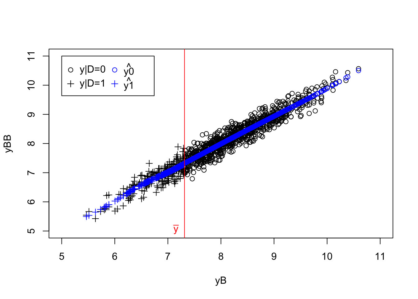
Figure 8.1: Placebo test with RDD LLR
Let us now estimate the resulting placebo parameter and its precision:
bw <- max(MSE.grid[MSE.llr.0==min(MSE.llr.0)],MSE.grid[MSE.llr.1==min(MSE.llr.1)])
yBB.h <- yBB[log(param['barY'])-bw<yB & yB<log(param['barY'])+bw]
Ds.h <- Ds[log(param['barY'])-bw<yB & yB<log(param['barY'])+bw]
yB.l <- (yB[log(param['barY'])-bw<yB & yB<log(param['barY'])+bw]-log(param['barY']))*Ds[log(param['barY'])-bw<yB & yB<log(param['barY'])+bw]
yB.r <- (yB[log(param['barY'])-bw<yB & yB<log(param['barY'])+bw]-log(param['barY']))*(1-Ds[log(param['barY'])-bw<yB & yB<log(param['barY'])+bw])
reg.rdd.local.ols <- lm(yBB.h ~ Ds.h + yB.l + yB.r)
TT.Placebo <- reg.rdd.local.ols$coef[2]
se.TT.Placebo <- sqrt(vcov(reg.rdd.local.ols)[2,2])
The estimated placebo treatment effect is of -0.05 \(\pm\) 0.09.
8.2.2.2 Testing the continuity of the density of the running variable around the threshold
McCrary (2008) has proposed a test of the continuity of the density of the running variable around the threshold. This test is one of the manipulation of the position around the threshold: maybe individuals are manipulating the value of their running variable in order to become eligible to the program. This would of course make the RDD estimate fully false.
The approach porposed by McCray has two steps:
- Build an undersmoothed histogram of the distribution of the running variable, using the selection threshold as a bound for two of the bins.
- Apply LLR on each side of the threshold and estimate the difference in the predicted value of the density at the threshold.
In order to build an histogram of the distribution of the running variable \(R_i\) around the selection threshold, McCrary proposes to build a discretized version of the running variable using the following transformation:
\[\begin{align*} g(R_i) & = \lfloor\frac{R_i-c}{b}\rfloor b+\frac{b}{2} + c, \end{align*}\]
with \(\lfloor a \rfloor\) the floor function, returning the greatest integer lower or equal to \(a\) (\(\lfloor a \rfloor = k\), with \(k\in\mathbf{Z}\) and \(k\leq a < k+1\)), \(c\) the selection threshold, and \(b\) the binsize. The \(g\) transformation generates a set of equi-spaced (with a distance \(b\)) values, \(X_1,X_2,\dots,X_J\) which serve as the \(x\)-axis of the histogram. The \(y\)-axis of the histogram is defined as the normalized number of observations that take each of these values:
\[\begin{align*} Y_j & = \frac{1}{Nb}\sum_{i=1}^N\uns{g(R_i)=X_j}. \end{align*}\]
The second step simply runs a LLR estimate through the resulting data \(\left(X_j,Y_j\right)\), around \(c\), yielding two estimates of the density, one above \(c\) (\(\hat{f}^+\)), and one below (\(\hat{f}^-\)). The final parameter estimate used to teste the continuity of the density of the running variable is \(\hat\theta\), with:
\[\begin{align*} \hat\theta & = \ln\hat{f}^+-\ln\hat{f}^-. \end{align*}\]
McCrary (2008) proves the following result:
Theorem 8.2 (Asymptotic distribution of the density disconuity estimator) If \(f\) has three continuous and bounded derivatives everywhere on its domain except at \(c\), if \(h\rightarrow 0\), \(Nh\rightarrow \infty\), \(\frac{b}{h}\rightarrow 0\) and \(h^2\sqrt{Nh}\rightarrow H\geq 0\) and if \(R_1,R_2,\dots,R_N\) is a random sample with density \(f\), we have:
\[\begin{align*} \sqrt{Nh}(\hat\theta-\theta) & \distr \mathcal{N}\left(B,\frac{24}{5}\left(\frac{1}{\hat{f}^+}+\frac{1}{\hat{f}^-}\right)\right). \end{align*}\]
Proof. See McCrary (2008).
Remark. Theorem 8.2 shows that the asymptotic distribution of \(\hat\theta\) is actually biased. This is a classical result of non-parametric statistics. The answer to that is to undersmooth, to make the bias term \(B\) go to zero faster than \(\sqrt{Nh}\), and therefore restores consistency. Undersmoothing means choosing a bandwidth \(h\) that is half the optimal bandwidth chosen by cross-validation.
Remark. Theorem 8.2 relies on a Local Linear Regression using the triangular kernel. We will use the Gaussian kernel in practice, and it should work fine.
Remark. In practice, McCrary (2008) suggests to use \(\hat{b}=\frac{2}{N}\hat{\sigma}\), with \(\hat{\sigma}\) the sample standard deviation of the running variable, and then to use as \(\hat{h}\) the average of the two quantities \(\kappa\left(\frac{\tilde{\sigma}^2(d-e)}{\sum_{j}\tilde{f''}(X_j)^2}\right)^{\frac{1}{5}}\), where \(d-e\) is \(X_J-c\) for the right-hand side regression and \(c-X_1\) for the left hand side, \(\kappa=3.348\), \(\tilde{\sigma}^2\) the mean squared error of a regression of a fourth order polynomial run on each side of the cutoff, and \(\tilde{f''}\) the second derivative estimate from this same regression.
Example 8.4 Let’s see how McCrary’s test works in our example. First, we have to build an undersmoothed histogram. For that, we need to choose a binsize \(b\) and generate the \(R_i\) variable. Let’s go.
# kernel
kernel = 'gaussian'
#threshold
c <- log(param["barY"])
# binwidth
b <- 0.05
# generating the discretized running variable
Data <- data.frame(yA,Ds,yB,yBB) %>%
        mutate(
          gR = floor((yB-c)/b)*b+b/2+c
        )
# generating the undersmoothed histogram
McCraryHist <- Data %>%
              group_by(gR,Ds) %>%
              summarize(
                Dens = n()/(N*b)
              ) %>%
              mutate(
                Ds = factor(Ds,levels=c("0","1"))
              )
# bandwidth choice by cross validation
MSE.grid <- seq(0.1,1,by=.1)
MSE.llr.0 <- sapply(MSE.grid,MSE.llr,y=McCraryHist$Dens,D=McCraryHist$Ds,x=McCraryHist$gR,kernel=kernel,d=0)
MSE.llr.1 <- sapply(MSE.grid,MSE.llr,y=McCraryHist$Dens,D=McCraryHist$Ds,x=McCraryHist$gR,kernel=kernel,d=1)
# LLR regression with optimal bandwidth
y0.llr <- llr(McCraryHist$Dens[McCraryHist$Ds==0],McCraryHist$gR[McCraryHist$Ds==0],McCraryHist$gR[McCraryHist$Ds==0],bw=MSE.grid[MSE.llr.0==min(MSE.llr.0)],kernel=kernel)
y1.llr <- llr(McCraryHist$Dens[McCraryHist$Ds==1],McCraryHist$gR[McCraryHist$Ds==1],McCraryHist$gR[McCraryHist$Ds==1],bw=MSE.grid[MSE.llr.1==min(MSE.llr.1)],kernel=kernel)
yLLR <- c(y1.llr,y0.llr)
McCraryHist$yLLR <- yLLR
# undersmoothing to estimate the actual effect
y0.llr.c <- llr(McCraryHist$Dens[McCraryHist$Ds==0],McCraryHist$gR[McCraryHist$Ds==0],c,bw=min(MSE.grid[MSE.llr.0==min(MSE.llr.0)],MSE.grid[MSE.llr.1==min(MSE.llr.1)])/2,kernel=kernel)
y1.llr.c <- llr(McCraryHist$Dens[McCraryHist$Ds==1],McCraryHist$gR[McCraryHist$Ds==1],c,bw=min(MSE.grid[MSE.llr.0==min(MSE.llr.0)],MSE.grid[MSE.llr.1==min(MSE.llr.1)])/2,kernel=kernel)
theta <- log(y1.llr.c)-log(y0.llr.c)
# estimating the standard error of theta
Se.theta <- 1/sqrt(N*min(MSE.grid[MSE.llr.0==min(MSE.llr.0)],MSE.grid[MSE.llr.1==min(MSE.llr.1)]))*sqrt((24/5)*(1/y1.llr.c+1/y0.llr.c))
Let’s plot the resulting data:
ggplot(McCraryHist,aes(x=gR,y=Dens)) +
  geom_point(shape=1) +
#  geom_point(aes(x=gR,y=yLLR),shape=2,color='blue')+
  geom_line(aes(x=gR,y=yLLR,group=Ds,color=Ds,linetype=Ds))+
  geom_vline(xintercept=c,color='red',linetype='dashed')+
  geom_text(x=c+0.05,y=-0.001,label=expression(bar('y')),color='red')+
  theme_bw()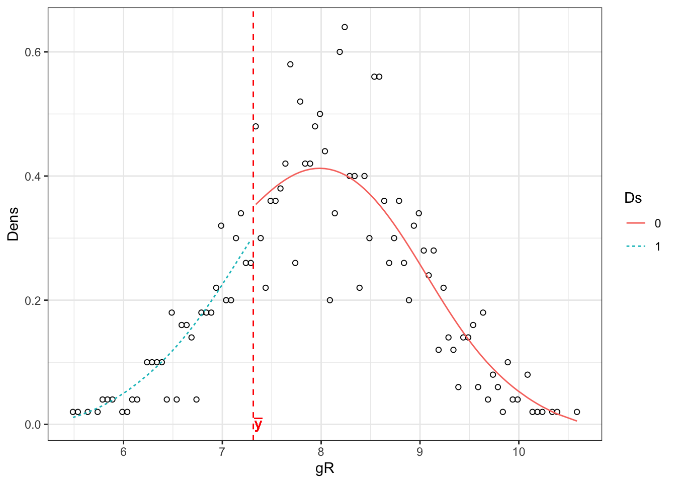
Figure 8.2: Histogram of the running variable
The resulting estimate is \(\hat\theta=\) -0.17 \(\pm\) 0.54.
8.2.3 Placebo tests for Difference in Differences
We are going to look at placebo tests for DID, DID-IV and staggered DID. The key assumptions we are going to test is the assumption of Parallel Trends (Assumption 4.14). We are actually going to test that this assumption holds in pre-treatment data. If it does, it will give more credence to the fact that it holds in the post-treatment period.
8.2.3.1 Testing for parallel trends in DID with two periods of pre-treatment data
With two years (\(BB\) and \(B\)) of pre-treatment data and knowledge of \(D_i\) (or \(Z_i\)) we can test the Parallel Trends Assumption by estimating the effect of a placebo treatment given on year \(B\) to the group with \(D_i=1\).
Example 8.5 Let’s see how this works in our example. For that, we are going to simiulate first a dataset with two periods of pre-treatment data.
Let us choose some parameter values first:
param <- c(8,.5,.28,1500,0.9,0.01,0.05,0.05,0.05,0.1)
names(param) <- c("barmu","sigma2mu","sigma2U","barY","rho","theta","sigma2epsilon","sigma2eta","delta","baralpha")
And generate some data:
N <- 1000
set.seed(1234)
mu <- rnorm(N,param["barmu"],sqrt(param["sigma2mu"]))
UBB <- rnorm(N,0,sqrt(param["sigma2U"]))
yBB <- mu + UBB
YBB <- exp(yBB)
epsilonB <- rnorm(N,0,sqrt(param["sigma2epsilon"]))
UB <- param["rho"]*UBB + epsilonB
yB <- mu + 0.5*param["delta"]+  UB
epsilonA <- rnorm(N,0,sqrt(param["sigma2epsilon"]))
U0A <- param["rho"]*UB + epsilonA
y0A <- mu +  U0A + param["delta"]
eta<- rnorm(N,0,sqrt(param["sigma2eta"]))
alpha <- param["baralpha"]+  param["theta"]*mu + eta
y1A <- y0A+alpha
Ds <- ifelse(yB<=log(param["barY"]),1,0)
yA <- y1A*Ds+y0A*(1-Ds)

y.t.1 <- c(mean(yBB[Ds==1]),mean(yB[Ds==1]),mean(yA[Ds==1]))
y.t.0 <- c(mean(yBB[Ds==0]),mean(yB[Ds==0]),mean(yA[Ds==0]))
y.did <- as.data.frame(c(y.t.1,y.t.0))
colnames(y.did) <- c('y')
y.did$time <- factor(c('BB','B','A','BB','B','A'),levels=c('BB','B','A'))
y.did$D <- factor(c(rep(1,3),rep(0,3)),levels=c(0,1))
Let us plot the resulting means:
ggplot(y.did, aes(x=time, y=y)) +
  geom_line(aes(colour=D,group=D)) +
  geom_point(aes(colour=D),size=3) +
  ylim(6,9) +
  theme_bw()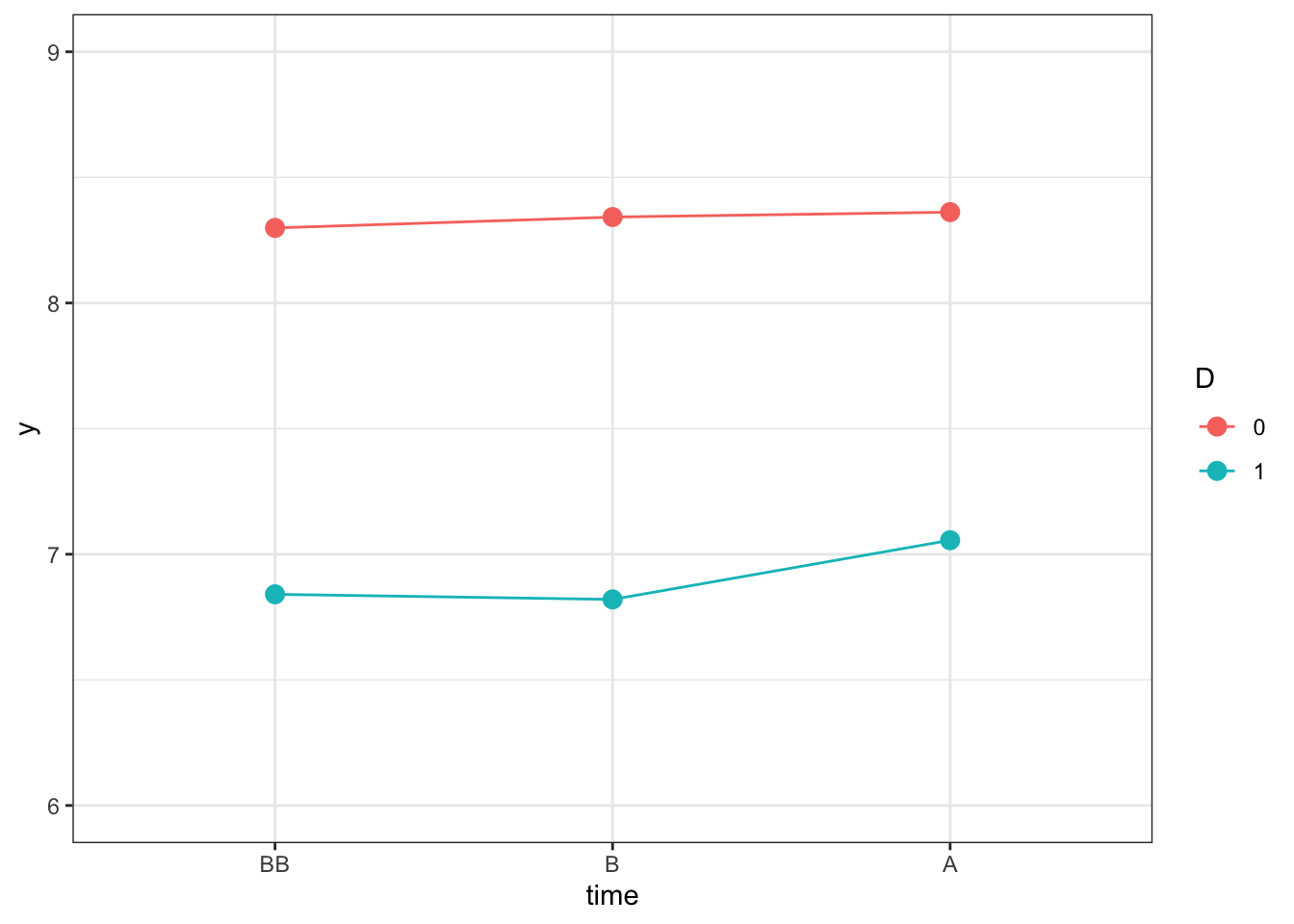
Figure 8.3: Outcomes Over Time in the Treated and Control Group
Let us now compute treatment effect estimates using \(B\) as our placebo treatment period. We are going to compare the estimates stemming from a pooled DID model (which ignores the individual level panel dimension of the data) and the fixed effects estimator.
y.pool <- c(yA,yB,yBB)
Ds.pool <- c(Ds,Ds,Ds)
time <- c(rep(2,N),rep(1,N),rep(0,N))
t.D <- time*Ds.pool
data.panel <- cbind(c(seq(1,N),seq(1,N),seq(1,N)),time,y.pool,Ds.pool,t.D)
colnames(data.panel) <- c('Individual','time','y','Ds','t.D')
data.panel <- as.data.frame(data.panel)
reg.did.pool <- lm(y ~ time + Ds + t.D,data=data.panel[data.panel$time<=1,])
reg.did.fe <- plm(y ~ time + t.D,data=data.panel[data.panel$time<=1,],index=c('Individual','time'),model='within')
placebo.did <- cbind(c(reg.did.fe$coef[2],reg.did.pool$coef[4]),c(sqrt(vcov(reg.did.fe)[2,2]),sqrt(vcov(reg.did.pool)[4,4])))
rownames(placebo.did) <- 1:nrow(placebo.did)
colnames(placebo.did) <- c('Coef','SeCoef')
placebo.did <- as.data.frame(placebo.did)
placebo.did$Method <- factor(c('FE','Pooled'),levels=c('Pooled','FE'))
Let’s plot our results:
ggplot(placebo.did, aes(x=Method, y=Coef)) +
  geom_pointrange(aes(ymin=Coef-1.96*SeCoef, ymax=Coef+1.96*SeCoef),position=position_dodge(.9),color='blue') +
  theme_bw()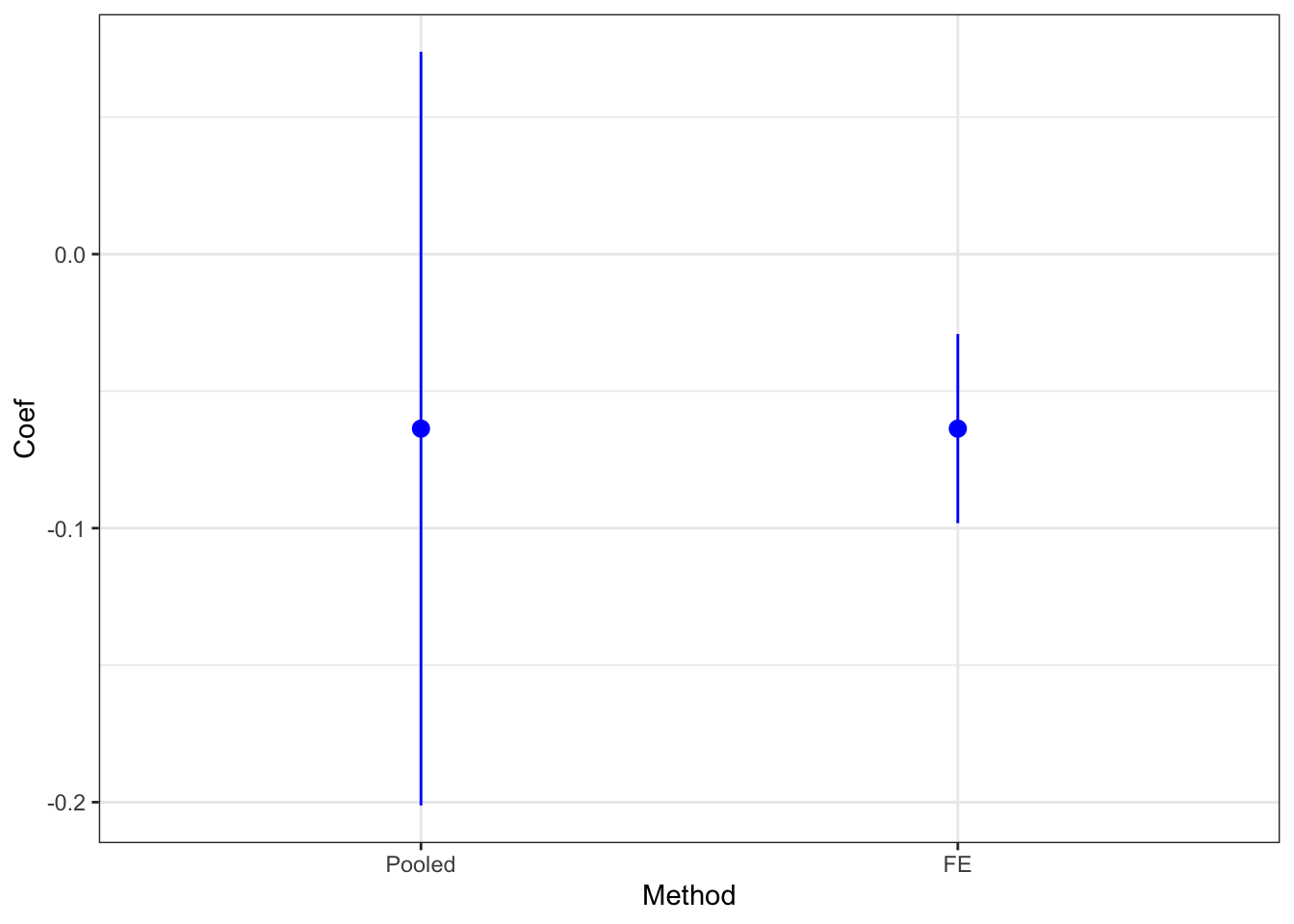
Figure 8.4: Placebo Test with DID
The estimated placebo effect with the fixed effects estimator is equal to -0.06 \(\pm\) 0.02. Therefore the test rejects the validity of DID. Why is that so? Remember that DID is valid in our model only when \(\rho=1\). This is absolutely not the case here, with \(\rho=\) 0.9.
8.2.3.2 Testing for parallel trends in DID-IV with two periods of pre-treatment data
In DID-IV, we are going to do the same test as with DID, except that we are going to use \(Z_i\) as the treatment group variable, as we are now testing the Parallel Trends Assumption 4.29.
Example 8.6 Let’s see how this works in our example: Let us first generate some data.
set.seed(1234)
N <-1000
# I am going to draw a state fixed effect for 50 states with variance 1/3 of the total variance of mu
Nstates <- 50
muS <- rnorm(Nstates,0,sqrt(param["sigma2mu"]/3))
muS <- rep(muS,each=N/Nstates)
# I draw an individual fixed effect with the remaining variance
muU <- rnorm(N,0,sqrt(param["sigma2mu"]*2/3))
mu <- param["barmu"] + muS + muU
UBB <- rnorm(N,0,sqrt(param["sigma2U"]))
yBB <- mu + UBB
YBB <- exp(yBB)
epsilonB <- rnorm(N,0,sqrt(param["sigma2epsilon"]))
UB <- param['rho']*UBB+epsilonB
yB <- mu + UB
YB <- exp(yB)
epsilon <- rnorm(N,0,sqrt(param["sigma2epsilon"]))
eta<- rnorm(N,0,sqrt(param["sigma2eta"]))
U0 <- param["rho"]*UB + epsilon
y0 <- mu +  U0 + param["delta"]
alpha <- param["baralpha"]+  param["theta"]*mu + eta
y1 <- y0+alpha
Y0 <- exp(y0)
Y1 <- exp(y1)

# Z=1 if states have lower muS than 0
Z <- ifelse(muS<=0,1,0)
Ds <- ifelse(YB<=param["barY"] & Z==1,1,0)
yA <- y1*Ds+y0*(1-Ds)
YA <- Y1*Ds+Y0*(1-Ds)

y.t.1 <- c(mean(yBB[Z==1]),mean(yB[Z==1]),mean(yA[Z==1]))
y.t.0 <- c(mean(yBB[Z==0]),mean(yB[Z==0]),mean(yA[Z==0]))
y.did.iv <- as.data.frame(c(y.t.1,y.t.0))
colnames(y.did.iv) <- c('y')
y.did.iv$time <- factor(c('BB','B','A','BB','B','A'),levels=c('BB','B','A'))
y.did.iv$Z <- factor(c(rep(1,3),rep(0,3)),levels=c(0,1))
Let us now plot the resulting estimates:
ggplot(y.did.iv, aes(x=time, y=y)) +
  geom_line(aes(colour=Z,group=Z)) +
  geom_point(aes(colour=Z),size=3) +
  ylim(6,9) +
  theme_bw()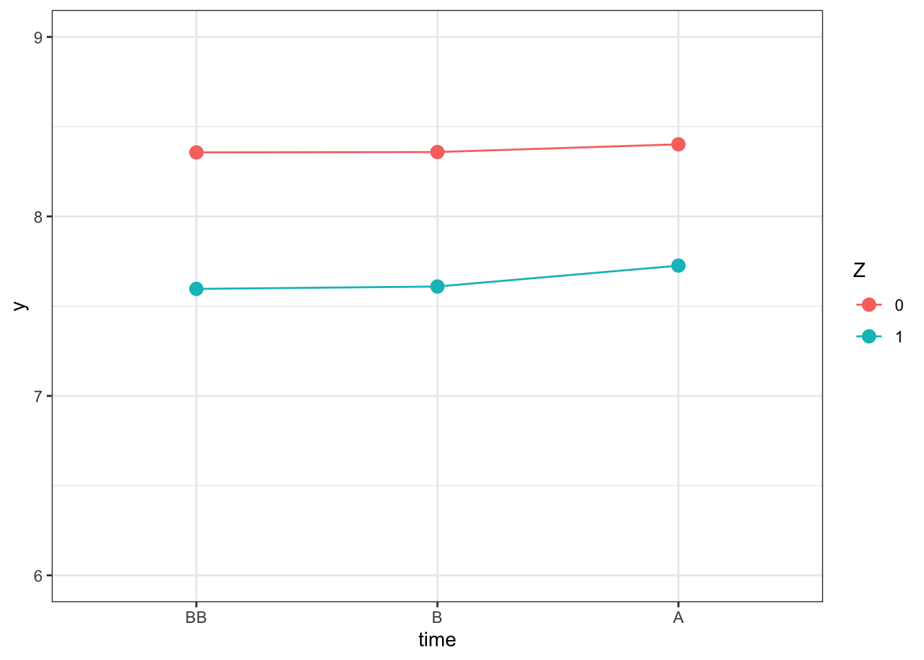
Figure 8.5: Outcomes Over Time
Let us now estimate the effect using the feols command of the fixest package, which will let us account for state-level autocorrelation between outcomes and the instrument, as we have seen in Chapter 9.
Let us first generate a dataset with all the required information.
DIDIVA <- data.frame(id=1:N,y=yA,Ds=Ds,Z=Z,time="A",muS=muS)
DIDIVB <- data.frame(id=1:N,y=yB,Ds=Ds,Z=Z,time="B",muS=muS)
DIDIVBB <- data.frame(id=1:N,y=yBB,Ds=Ds,Z=Z,time="BB",muS=muS)
DIDIVPlacebo <- rbind(DIDIVA,DIDIVB,DIDIVBB) %>%
              # Adding a treatment indicator taking value Ds when period is B and zero otherwise
              mutate(
                ZPlacebo = case_when(
                  time == "B" ~ Z,
                  time != "B" ~ 0
                ),
                DPlacebo = case_when(
                  time == "B" ~ Ds,
                  time != "B" ~ 0
                )
              ) %>%
              # Adding a State level indicator for clustering
              group_by(muS) %>%
              mutate(
                StateId = cur_group_id()
              )
Let us now estimate the model on the placebo periods \(t=B\) and \(t=BB\):
# running DID regression on Placebo Z
regDIDIVPlacebo <- feols(y ~ ZPlacebo | time + id,data=filter(DIDIVPlacebo,time!="A"),cluster="StateId")
PlaceboDIDIVCoef <- coef(regDIDIVPlacebo)[[1]]
PlaceboDIDIVSe <- sqrt(diag(vcov(regDIDIVPlacebo))[[1]])
# running DID regression on Placebo D
regDIDPlacebo <- feols(y ~ DPlacebo | time + id,data=filter(DIDIVPlacebo,time!="A"),cluster="StateId")
PlaceboDIDCoef <- coef(regDIDPlacebo)[[1]]
PlaceboDIDSe <- sqrt(diag(vcov(regDIDPlacebo))[[1]])
When testing the Parallel Trends Assumption on the instrumental variable \(Z_{i}\), we find a placebo Intention to Treat Effect of 0.01 \(\pm\) 0.02. When using the treatment indicator directly, instead, the placebo test of DID yields a placebo Treatment Effect on the Treated of -0.02 \(\pm\) 0.04.
8.2.3.3 Testing for parallel trends in DID with multiple periods of pre-treatment data
When we have access to several years of pre-treatment data, we can theoretically conduct several placebo tests: one for each additional pre-treatment year on top of the reference year. In staggered designs, this is compounded by the fact that we can conduct one such placebo test per cohort. The usual practice, in traditional non-staggered DID designs with multiple periods, is to consider that the placebo test is valid when none of the pre-treatment placebo tests is statistically significantly different from zero at usual levels of significance. There might be some visual tolerance if one of the effects is slightly significant. With staggered designs, there is no established practice yet, but it seems that people look at the placebo estimates aggregated over all cohorts in order to judge the quality of the test. A more severe test would look at each of the individual cohort estimates and have them to be non zero.
Example 8.7 Let’s see how this works in practice, with the example of staggered designs. In order to see what happens let’s first generate some data:
param <- c(8,.5,.28,1500,0.9,
           0.01,0.01,0.01,0.01,
           0.05,0.05,
           0,0.1,0.2,0.3,
           0.05,0.1,0.15,0.2,
           0.25,0.1,0.05,0,
           1.5,1.25,1,0.75,
           0.5,0,-0.5,-1,
           0.1,0.28,0)
names(param) <- c("barmu","sigma2mu","sigma2U","barY","rho",
                  "theta1","theta2","theta3","theta4",
                  "sigma2epsilon","sigma2eta",
                  "delta1","delta2","delta3","delta4",
                  "baralpha1","baralpha2","baralpha3","baralpha4",
                  "barchi1","barchi2","barchi3","barchi4",
                  "kappa1","kappa2","kappa3","kappa4",
                  "xi1","xi2","xi3","xi4",
                  "gamma","sigma2omega","rhoetaomega")
Let us now generate the corresponding data (in long format):
set.seed(1234)
N <- 1000
T <- 4
cov.eta.omega <- matrix(c(param["sigma2eta"],param["rhoetaomega"]*sqrt(param["sigma2eta"]*param["sigma2omega"]),param["rhoetaomega"]*sqrt(param["sigma2eta"]*param["sigma2omega"]),param["sigma2omega"]),ncol=2,nrow=2)
data <- as.data.frame(mvrnorm(N*T,c(0,0),cov.eta.omega))
colnames(data) <- c('eta','omega')
# time and individual identifiers
data$time <- c(rep(1,N),rep(2,N),rep(3,N),rep(4,N))
data$id <- rep((1:N),T)
# unit fixed effects
data$mu <- rep(rnorm(N,param["barmu"],sqrt(param["sigma2mu"])),T)
# time fixed effects
data$delta <- c(rep(param["delta1"],N),rep(param["delta2"],N),rep(param["delta3"],N),rep(param["delta4"],N))
data$baralphat <- c(rep(param["baralpha1"],N),rep(param["baralpha2"],N),rep(param["baralpha3"],N),rep(param["baralpha4"],N))

# building autocorrelated error terms
data$epsilon <- rnorm(N*T,0,sqrt(param["sigma2epsilon"]))
data$U[1:N] <- rnorm(N,0,sqrt(param["sigma2U"]))
data$U[(N+1):(2*N)] <- param["rho"]*data$U[1:N] + data$epsilon[(N+1):(2*N)]
data$U[(2*N+1):(3*N)] <- param["rho"]*data$U[(N+1):(2*N)] + data$epsilon[(2*N+1):(3*N)]
data$U[(3*N+1):(T*N)] <- param["rho"]*data$U[(2*N+1):(3*N)] + data$epsilon[(3*N+1):(T*N)]
# potential outcomes in the absence of the treatment
data$y0 <- data$mu + data$delta + data$U
data$Y0 <- exp(data$y0)
# treatment timing
# error term
data$V <- param["gamma"]*(data$mu-param["barmu"])+data$omega
# treatment group, with 99 for the never treated instead of infinity
Ds <- if_else(data$y0[1:N]+param["xi1"]+data$V[1:N]<=log(param["barY"]),1,
              if_else(data$y0[1:N]+param["xi2"]+data$V[1:N]<=log(param["barY"]),2,
                      if_else(data$y0[1:N]+param["xi3"]+data$V[1:N]<=log(param["barY"]),3,
                              if_else(data$y0[1:N]+param["xi4"]+data$V[1:N]<=log(param["barY"]),4,99))))
data$Ds <- rep(Ds,T)
# Treatment status
data$D <- if_else(data$Ds>data$time,0,1)
# potential outcomes with the treatment
# effect of the treatment by group
data$baralphatd <- if_else(data$Ds==1,param["barchi1"],
                           if_else(data$Ds==2,param["barchi2"],
                                   if_else(data$Ds==3,param["barchi3"],
                                           if_else(data$Ds==4,param["barchi4"],0))))+
                  if_else(data$Ds==1,param["kappa1"],
                           if_else(data$Ds==2,param["kappa2"],
                                   if_else(data$Ds==3,param["kappa3"],
                                           if_else(data$Ds==4,param["kappa4"],0))))*(data$t-data$Ds)*if_else(data$time>=data$Ds,1,0)
data$y1 <- data$y0 + data$baralphat + data$baralphatd + if_else(data$Ds==1,param["theta1"],if_else(data$Ds==2,param["theta2"],if_else(data$Ds==3,param["theta3"],param["theta4"])))*data$mu + data$eta
data$Y1 <- exp(data$y1)
data$y <- data$y1*data$D+data$y0*(1-data$D)
data$Y <- data$Y1*data$D+data$Y0*(1-data$D)
Let’s now estimate Sun and Abraham’s model:
# regression
reg.fixest.SA.Agg <- feols(y ~ sunab(Ds,time)| id + time, data=filter(data,Ds>1),cluster='id')

# Disaggregate estimates
disaggregate.SA <- as.data.frame(cbind(coef(reg.fixest.SA.Agg,agg=FALSE),se(reg.fixest.SA.Agg,agg=FALSE)))
colnames(disaggregate.SA) <- c('Coef','Se')
# adding treatment groups and time to treatment
disaggregate.SA <- disaggregate.SA %>%
                    mutate(test =  names(coef(reg.fixest.SA.Agg,agg=FALSE))) %>%
                    mutate(
                      Group = factor(str_sub(test,-1),levels=c('1','2','3','4','Aggregate')),
                      TimeToTreatment = factor(if_else(str_detect(test,"\\-"),str_extract(test,"\\-[[:digit:]]"),str_extract(test,"[[:digit:]]")),levels=c('-3','-2','-1','0','1','2'))
                    ) %>%
                  select(-test)

# adding reference period
Group <- c('2','3','4')
TimeToTreatment <- rep('-1',3)
ref.dis <- as.data.frame(cbind(Group,TimeToTreatment)) %>%
        mutate(
          Coef = 0,
          Se = 0,
          Group = factor(Group,levels=c('1','2','3','4','Aggregate')),
          TimeToTreatment = factor(TimeToTreatment,levels=c('-3','-2','-1','0','1','2'))
          )
disaggregate.SA <- rbind(disaggregate.SA,ref.dis)

# adding aggregate results
# aggregate estimates
aggregate.SA <- as.data.frame(cbind(coef(reg.fixest.SA.Agg),se(reg.fixest.SA.Agg)))
colnames(aggregate.SA) <- c('Coef','Se')
# adding treatment groups and time to treatment
aggregate.SA <- aggregate.SA %>%
                    mutate(test =  names(coef(reg.fixest.SA.Agg))) %>%
                    mutate(
                      Group = factor(rep("Aggregate",5),levels=c('1','2','3','4','Aggregate')),
                      TimeToTreatment = factor(if_else(str_detect(test,"\\-"),str_extract(test,"\\-[[:digit:]]"),str_extract(test,"[[:digit:]]")),levels=c('-3','-2','-1','0','1','2'))
                    ) %>%
                  select(-test)

# adding reference period
Group <- c("Aggregate")
TimeToTreatment <- rep('-1',1)
ref <- as.data.frame(cbind(Group,TimeToTreatment)) %>%
        mutate(
          Coef = 0,
          Se = 0,
          Group = factor(Group,levels=c('1','2','3','4','Aggregate')),
          TimeToTreatment = factor(TimeToTreatment,levels=c('-3','-2','-1','0','1','2'))
          )
disaggregate.SA <- rbind(disaggregate.SA,aggregate.SA,ref) %>%
mutate(TimeToTreatment = as.numeric(as.character(TimeToTreatment)))ggplot(disaggregate.SA %>% filter(TimeToTreatment<0),aes(x=TimeToTreatment,y=Coef,colour=Group,linetype=Group))+
geom_line() +
geom_pointrange(aes(ymin=Coef-1.96*Se,ymax=Coef+1.96*Se),position=position_dodge(0.1)) +
ylab("DID estimate") +
xlab("Time relative to treatment") +
scale_x_continuous(breaks=c(-3,-2,-1,0,1,2)) +
expand_limits(y=0) +
scale_colour_discrete(name="Treatment\ngroup")+
scale_linetype_discrete(name="Treatment\ngroup")+
theme_bw()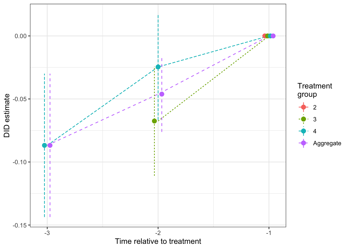
Figure 8.6: Placebo tests for DID estimated using Sun and Abraham procedure (reference period \(\tau'=1\))
As we can see on Figure 8.6, the placebo test for the group that enters the treatment at period 4 is significantly different from zero (it is equal to -0.09 \(\pm\) 0.06). In this case, we would reject the parallel trends assumption, and we would be correct. There are non parallel trends in our model because of regression to the mean.
8.3 Placebo tests for observational methods
It might seem strange to think of testing the validity of observational methods without additional data. Indeed, observational methods work mostly by assuming that conditioning on everything that we observe pre-treatment is what is required to cancel selection bias. How could we ever find variables that we would use for placebo tests, that we would not like to condition on in the first place? One proposal has been made by Imbens and Wooldridge (2009): measure the effect of the treatment on outcomes observed at \(t=k-1\), where \(k\) is the actual treatment date, by conditioning on \(Y_{i,k-2}\) and other pre-treatment covariates. If the matching estimator is able to find a zero treatment effect, you would have a confirmation that your approach works. What we are going to see here is that this approach is actually misguided: unless there is no selection bias at all (which we can easily check), it is going to reject cases where the matching estimator is perfectly valid. Here, I am proposing to run the reverse test: estimate the effect on \(Y_{i,k-2}\) conditioning on \(Y_{i,k-1}\). This test will not reject when matching is correct, and will have the same rejection properties when matching is not correct.
Here is a quick theoretical argument of why Imbens and Wooldridge (2009)’s proposal is flawed and why my alternative proposal works. The reasoning and model I’m using are derived from my own research, namely Chabe-Ferret (2015). To make things simpler, let’s assume that we have only selection on transitory shocks (there are no permanent fixed effects). In that case, we have:
\[\begin{align*} Y^0_{i,t} & = \rho Y^0_{i,t-1} + U_{i,t} \\ D_{i,k} & = \uns{Y^0_{i,k-1}+V_{i,k}\leq 0}, \end{align*}\]
with \(V_{i,k}\) a shock independent of all the other shocks in the model.
In that model, we can show the following theorem:
Theorem 8.3 (Placebo tests for matching) In the simplified model where there is only selection on transitory shocks, Matching is unbiased, Imbens and Wooldridge (2009)’s test rejects the validity of matching and my proposed reversed test accepts the validity of matching:
\[\begin{align*} \Delta^{Y_{k+\tau}}_{M}(Y_{k-1}) & = \Delta^{Y_{k+\tau}}_{TT} \\ \Delta^{Y_{k-1}}_{M}(Y_{k-2}) & \neq 0 \\ \Delta^{Y_{k-2}}_{M}(Y_{k-1}) & = 0, \end{align*}\]
with \(\Delta^{Y_{k+\tau}}_{M}(Y_{k-\tau'})=\esp{Y_{i,k+\tau}-\esp{Y_{i,k+\tau}|Y_{i,k-\tau'},D_{i,k}=0}|D_{i,k}=1}\) the matching estimator for the effect at period \(k+\tau\) conditioning on \(Y_{i,k-\tau'}\).
Proof. Because \(V_{i,k}\) is independent from all the other shocks in the model, conditioning on \(Y_{i,k-1}\) is sufficient to get rid of selection bias:
\[\begin{align*} \esp{Y^0_{i,k+\tau}|D_{i,k}=1,Y_{i,k-1}} & = \esp{Y^0_{i,k+\tau}|Y_{i,k-1}} \\ & = \esp{Y^0_{i,k+\tau}|D_{i,k}=0,Y_{i,k-1}}. \end{align*}\]
This, together with the Law of Iterated Expectations, proves the first part of the theorem. Now, let’s look at what Imbens and Wooldridge (2009)’s test does. It computes the placebo treatment effect \(\Delta^{Y_{k-1}}_{M}(Y_{k-2})\) as:
\[\begin{align*} \Delta^{Y_{k-1}}_{M}(Y_{k-2}) & = \esp{Y^0_{i,k-1}|D_{i,k}=1,Y_{i,k-2}} -\esp{Y^0_{i,k-1}|D_{i,k}=0,Y_{i,k-2}}\\ & = \esp{\rho Y^0_{i,k-2} + U_{i,k-1}|D_{i,k}=1,Y_{i,k-2}} -\esp{\rho Y^0_{i,k-2} + U_{i,k-1}|D_{i,k}=0,Y_{i,k-2}}\\ & = \esp{U_{i,k-1}|D_{i,k}=1,Y_{i,k-2}} -\esp{U_{i,k-1}|D_{i,k}=0,Y_{i,k-2}}\\ & = \esp{U_{i,k-1}|D_{i,k}=1} -\esp{U_{i,k-1}|D_{i,k}=0}\\ & = \esp{U_{i,k-1}|Y^0_{i,k-1}+V_{i,k}\leq 0} -\esp{U_{i,k-1}|Y^0_{i,k-1}+V_{i,k}> 0}\\ & = \esp{U_{i,k-1}|U_{i,k-1}+\rho Y^0_{i,k-2}+V_{i,k}\leq 0} -\esp{U_{i,k-1}|U_{i,k-1}+\rho Y^0_{i,k-2}+V_{i,k}> 0}\\ & \neq 0, \end{align*}\]
where the first equality is definitional, the second equality uses the model, the third equality uses the fact that \(Y^0_{i,k-2}=Y_{i,k-2}\) and \(\esp{Y^0_{i,k-2}|D_{i,k},Y_{i,k-2}}=Y_{i,k-2}\), the fourth equality uses the fact that \(U_{i,k-1}\) is independent from \(Y_{i,k-2}\) and the fifth and sixth equalities use the model. The result follows because, since \(Y^0_{i,k-2}\) and \(V_{i,k}\) are independent from \(U_{i,k-1}\), the final expectations of \(U_{i,k-1}\) are conditional on a variable positively correlated with \(U_{i,k-1}\) to be above or below a threshold, which cannot be equal to zero. Indeed, since \(\esp{U_{i,k-1}}=0\), \(\esp{U_{i,k-1}|U_{i,k-1}+\rho Y^0_{i,k-2}+V_{i,k}\leq 0}< 0\) and \(\esp{U_{i,k-1}|U_{i,k-1}+\rho Y^0_{i,k-2}+V_{i,k}\leq 0}> 0\), hence the result.
Let’s see how my proposed test works in that case:
\[\begin{align*} \Delta^{Y_{k-2}}_{M}(Y_{k-1}) & = \esp{Y^0_{i,k-2}|D_{i,k}=1,Y_{i,k-1}} -\esp{Y^0_{i,k-2}|D_{i,k}=0,Y_{i,k-1}}\\ & = \esp{Y^0_{i,k-2}|Y^0_{i,k-1}+V_{i,k}\leq 0,Y_{i,k-1}} -\esp{Y^0_{i,k-2}|Y^0_{i,k-1}+V_{i,k}> 0,Y_{i,k-1}}\\ & = \esp{Y^0_{i,k-2}|Y_{i,k-1}} -\esp{Y^0_{i,k-2}|Y_{i,k-1}}\\ & = 0, \end{align*}\]
where the first equality is definitional, the second equality uses the model and the third equality uses the fact that \(V_{i,k}\) is independent from all the other variables in the model, and therefore independent from \(Y^0_{i,k-2}\), even after conditioning on \(Y^0_{i,k-1}\) (this actually uses Lemma 4.2 in Dawid (1979)). This proves the result.
Remark. Theorem 1 in Chabe-Ferret (2017) shows that the simple model we have written is the only one where matching is going to be consistent. Coupled with Theorem 8.3, this means that Imbens and Wooldridge (2009)’s test will always reject in all the cases when matching is consistent. My proposed test, on the contrary, will accept the validity of matching everytime it is consistent, and will reject when it is not.
Example 8.8 Let’s see how both of these tests work in our example. For that, we need to generate data with at least three pre-treatment periods. Let us first choose a simple model, with \(k\) the date at which treatment starts:
\[\begin{align*} y^0_{i,t} & = \bar\mu + \delta_t+U^0_{i,t} \\ U^0_{i,t} & = \rho U^0_{i,t-1}+\epsilon_{i,t} \\ D_{i,k} & = \uns{y^0_{i,k-1}+ \xi_k + V_i\leq\bar{y}} \\ V_i & = \sim\mathcal{N}(0,\sigma^2_{V}) \\ U^0_{i,1} & \sim\mathcal{N}(0,\sigma^2_{U}) \\ \epsilon_{i,t} & \sim\mathcal{N}(0,\sigma^2_{\epsilon}), \end{align*}\]
Let us now choose some parameter values:
param <- c(8,.28,0.28,1500,0.9,0.05,
           0,0.1,0.2,0.3,
           0.5,0,-0.5,-1)
names(param) <- c("barmu","sigma2U","sigma2V","barY","rho","sigma2epsilon",
                  "delta1","delta2","delta3","delta4",
                  "xi1","xi2","xi3","xi4")
Let us now generate some data, with \(k=4\):
set.seed(1234)
N <- 1000
T <- 4
data <- data.frame(time=c(rep(1,N),rep(2,N),rep(3,N),rep(4,N)),id=rep((1:N),T))
# time fixed effects
data$delta <- c(rep(param["delta1"],N),rep(param["delta2"],N),rep(param["delta3"],N),rep(param["delta4"],N))

# building autocorrelated error terms
data$epsilon <- rnorm(N*T,0,sqrt(param["sigma2epsilon"]))
data$U[1:N] <- rnorm(N,0,sqrt(param["sigma2U"]))
data$U[(N+1):(2*N)] <- param["rho"]*data$U[1:N] + data$epsilon[(N+1):(2*N)]
data$U[(2*N+1):(3*N)] <- param["rho"]*data$U[(N+1):(2*N)] + data$epsilon[(2*N+1):(3*N)]
data$U[(3*N+1):(T*N)] <- param["rho"]*data$U[(2*N+1):(3*N)] + data$epsilon[(3*N+1):(T*N)]
# potential outcomes in the absence of the treatment
data$y0 <- param["barmu"] + data$delta + data$U
# treatment timing
# error term
V <- rnorm(N,0,sqrt(param["sigma2V"]))
# Let's focus only on the treatment given at period 4
Ds <- if_else(data$y0[which(data$time==3)]+param["xi4"]+V<=log(param["barY"]),1,0)
data$Ds <- rep(Ds,T)
# let's put the data in wide format now
data <- data %>%
        select(id,time,y0,Ds) %>%
        pivot_wider(names_from="time",values_from = "y0",names_prefix = "y")
Let us first check that matching is indeed consistent in this dataset.
We are going to use the Matching package for that.
NNM.Match.y4.y3 <- Match(data$y4,data$Ds,data$y3,estimand='ATT',M=1,replace=TRUE,CommonSupport = FALSE,Weight=1,Var.calc=1,sample=FALSE)
ATT.y40.y3 <- NNM.Match.y4.y3$est
ATT.y40.y3.se <- NNM.Match.y4.y3$se
We find that \(\hat\Delta^{y^0_{4}}_{M}(y_{3})=\) -0.023 \(\pm\) 0.04. Let us now estimate Imbens and Wooldridge (2009)’s placebo test:
NNM.Match.y3.y2 <- Match(data$y3,data$Ds,data$y2,estimand='ATT',M=1,replace=TRUE,CommonSupport = FALSE,Weight=1,Var.calc=1,sample=FALSE)
ATT.y30.y2 <- NNM.Match.y3.y2$est
ATT.y30.y2.se <- NNM.Match.y3.y2$se
We find that \(\hat\Delta^{y^0_{3}}_{M}(y_{2})=\) -0.157 \(\pm\) 0.052. Let us now estimate my proposed placebo test:
NNM.Match.y2.y3 <- Match(data$y2,data$Ds,data$y3,estimand='ATT',M=1,replace=TRUE,CommonSupport = FALSE,Weight=1,Var.calc=1,sample=FALSE)
ATT.y20.y3 <- NNM.Match.y2.y3$est
ATT.y20.y3.se <- NNM.Match.y2.y3$se
We find that \(\hat\Delta^{y^0_{2}}_{M}(y_{3})=\) 0.006 \(\pm\) 0.064.