Nudging participation in the Conservation Reserve Program in the US
Wallander et al (2017) present the results of a large-scale field experiment within the USDA’s Conservation Reserve Program (CRP) that examines whether informational outreach, including behavioral nudges, could improve land owners’ willingness to participate. The experiment evaluates the impact of three types of reminder letters on the rate at which land is offered into the CRP.
Treatment 1, the basic treatment, consists of an informational letter that reminds farmers about the General Signup and their eligibility for the program. The key behavioral insight embedded in the letter is a reminder that the General Sign-up period had begun.
Treatment 2 keeps the same content as treatment 1 and adds a side box that told farmers how other stewards in their state had provided ecosystem services for their neighbors through participation in CRP, suggesting the popularity of CRP.
Treatment 3 augments treatment 2 by adding two boxes, both of which signal to farmers the private benefits of enrolling in CRP. The first box emphasizes the stability of CRP payments. The second box uses a peer comparison to signal the regional popularity of CRP.
There are two treatment groups in this experiment: the group of farmers with expiring contracts and the group of previously unenrolled farmers.


Impact and cost-effectiveness of the treatments
The main results of the paper are:
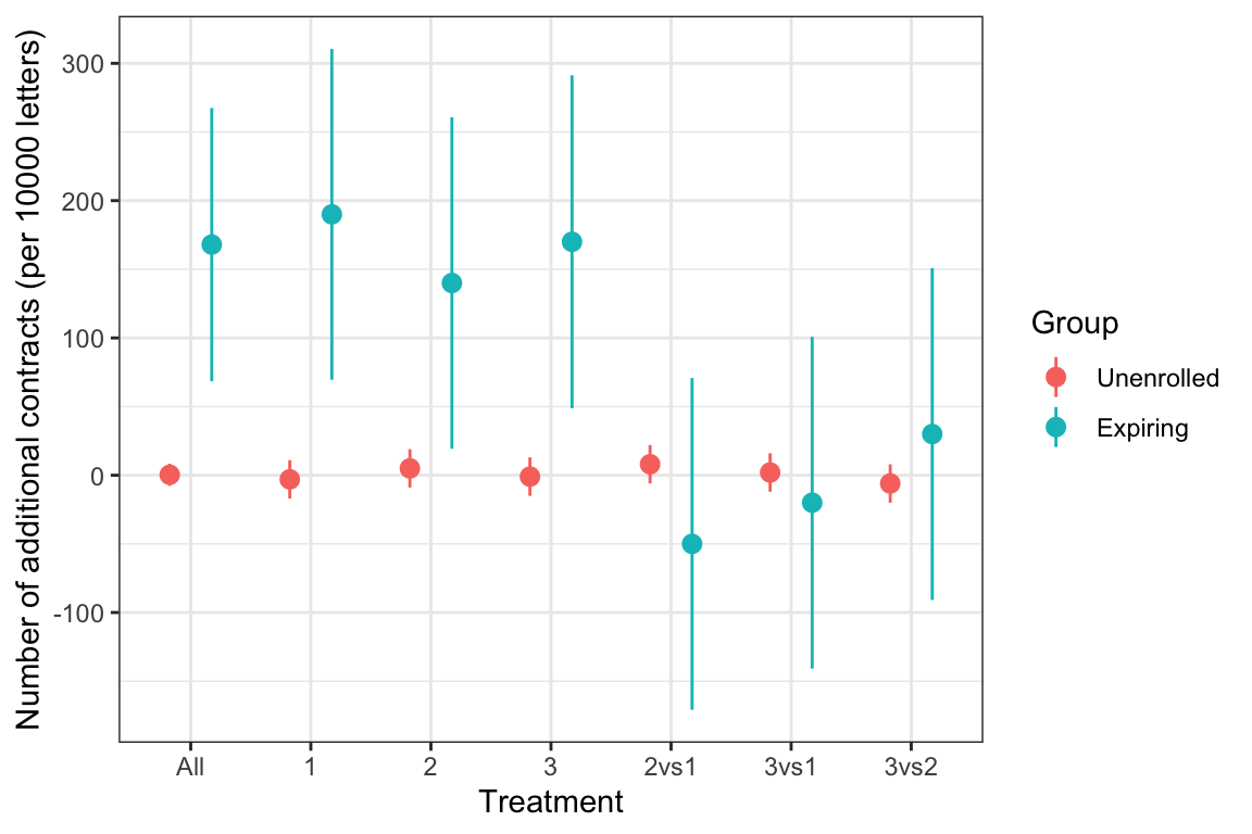
- The nudges did not have any detectable effect on enrollment in the group of previously unenrolled farmers. The estimated null effect is very precise (0 \(\pm\) 8 contract applications per 10000 letters).
- The nudges did have a detectable effect on the group of farmers with an expiring contract, but the effect is less precise (168 \(\pm\) 102 contract applications per 10000 letters).
- There is no discernable impact of the additional nudges on top of the simple letter in the group of farmers with an expiring contract.
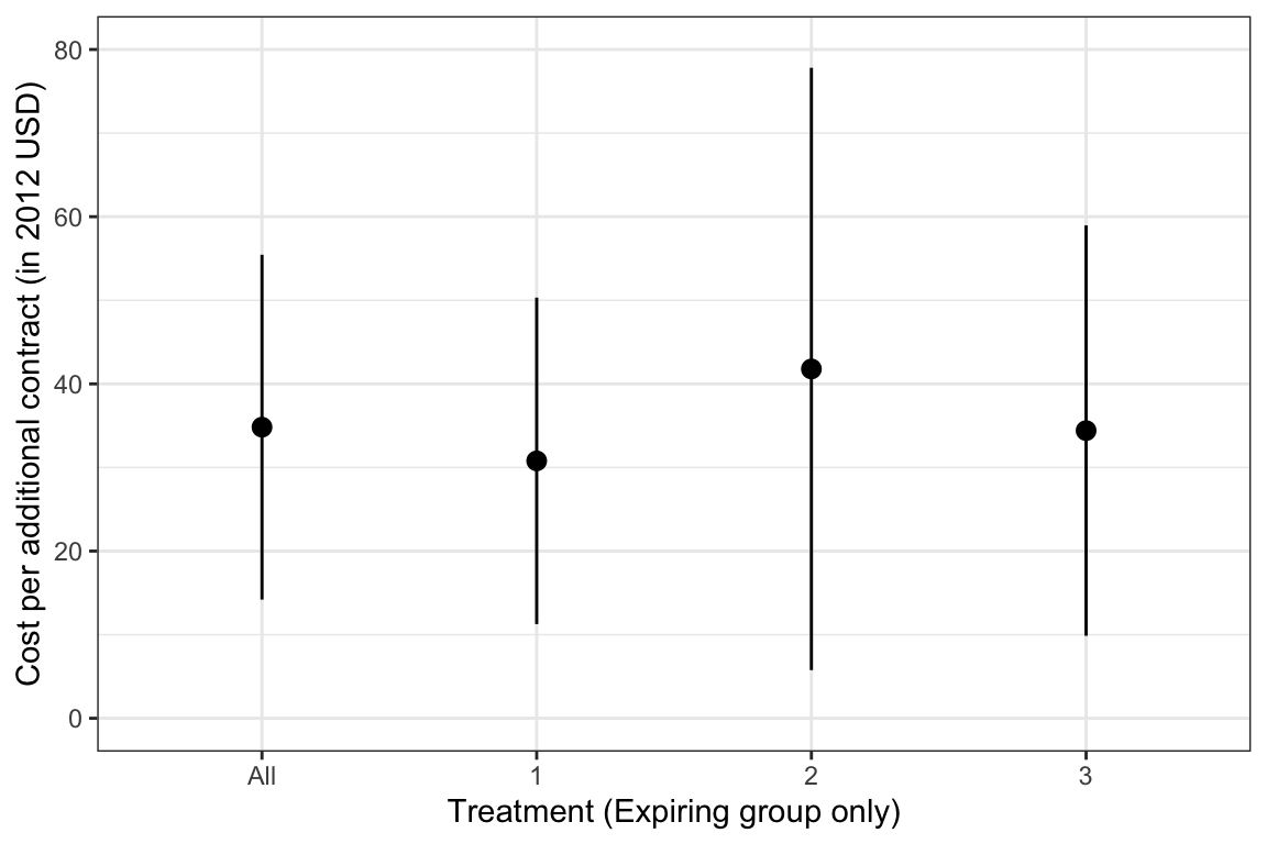
- The cost of an additional application is 35 \(\pm\) 22 2012USD in the group of farmers with an expiring contract.
Below is how we extracted these results from the paper.
Results for the group of farmers with expiring contracts
Offer rates are 0.575 in the control group and 0.594, 0.589, and 0.591 in the three treatment arms. The differences in offer rates from the control group (and thus the estimated causal effects from the three treatments) are 1.9, 1.4, and 1.7 percentage points, respectively. Each treatment effect is statistically significantly different from zero; the \(p-\)values for the three treatment effects are 0.002, 0.023, and 0.006 for treatments 1, 2, and 3, respectively.
Given that there is no statistical difference between treatments, if we pool all three treatments the offer rate among all high-information farms receiving a letter is 0.591, indicating that the treatment effect of receiving any letter is an increase in the offer rate of 1.68 percentage points. The 95% confidence interval for the pooled treatment effect is 0.69 to 2.68 percentage points.
We convert the precision estimates in standard deviations by inverting the \(p-\)values or the confidence intervals. For a 2-sided t-test, the \(p-\)value is equal to: \(p=2(1-\Phi(|\frac{\hat\beta}{\hat\sigma_{\beta}}|))\), with \(\Phi\) the c.d.f. of the standard normal distribution and \(\hat\sigma_{\beta}\) the standard error of the estimated treatment effect. As a consequence, for a positive effect, we can estimate the standard error as: \(\hat\sigma_{\beta}=\frac{\hat\beta}{\Phi^{-1}(1-\frac{p}{2})}\). If \(\bar{\beta}_{\alpha}\) and \(\underline{\beta}_{\alpha}\) are the two extremities of the \(100\alpha\)% confidence interval, we know that \(\hat\sigma_{\beta}=\frac{\bar{\beta}_{\alpha}-\underline{\beta}_{\alpha}}{2\Phi^{-1}(\frac{1+\alpha}{2})}\) (when both extremities are positive).
Let us wrap these results in a table.
# function for inverting p-values
se.pval <- function(pval,beta){
  return(beta/qnorm(1-pval/2))
}
# function for inverting confidence intervals
se.CI <- function(alpha,betalow,betahigh){
  return((betahigh-betalow)/(2*qnorm((1+alpha)/2)))
}

# treatment effects
wall.exp.TE <- c(1.68,1.9,1.4,1.7)
names(wall.exp.TE) <- c("All","1","2","3")

# relative effects
wall.exp.TE[5:7] <- c(1.4-1.9,1.7-1.9,1.7-1.4)
names(wall.exp.TE)[5:7] <- c("2vs1","3vs1","3vs2")

# pvalues
wall.exp.pval <- c(0.002,0.023,0.006)
names(wall.exp.pval) <- c("1","2","3")

# confidence interval
wall.exp.CI <- c(0.69,2.68)
names(wall.exp.CI) <- c("AllLow","AllHigh")

# computing precision
wall.exp.se <- c(0,0,0,0,0,0,0)
names(wall.exp.se) <- c("All","1","2","3","2vs1","3vs1","3vs2")

wall.exp.se[[1]] <- se.CI(alpha=0.95,betalow=wall.exp.CI[[1]],betahigh=wall.exp.CI[[2]])
wall.exp.se[2:4] <- purrr::map2_dbl(wall.exp.pval,wall.exp.TE[2:4],se.pval)
# we give the mean precision of the individual treatment effects to the relative effects
wall.exp.se[5:7] <- mean(wall.exp.se[2:4])

# putting results together in a dataframe
wall.exp <- as.data.frame(cbind(wall.exp.TE,wall.exp.se))
colnames(wall.exp) <- c('TE','SeTE')
wall.exp$Treatment <- c("All","1","2","3","2vs1","3vs1","3vs2")
wall.exp$Group <- "Expiring"
Results for the group of previously unenrolled farmers.
Among the previously unenrolled farmers, offer rates are 0.0022 in the control group and 0.0019, 0.0027 and 0.0021 in the three treatment arms. The differences in offer rates from the control group (and thus the estimated causal effects from the three treatments) are -0.03, 0.05 and -0.01 percentage points, respectively. The precision of this experiment is not given in the text. We simply know that this experiment had sufficient power to detect an approximate doubling of the offer rate, from 0.2% to 0.4%. We know that, for a two-sided t-test of level \(\alpha\), the power is equal to \(\kappa=\Phi(|\frac{\hat\beta}{\hat\sigma_{\beta}}|-\Phi^{-1}(1-\frac{\alpha}{2}))\). As a consequence, we can approximate the standard error of the treatment effect by \(\hat\sigma_{\beta}=\frac{\hat\beta}{\Phi^{-1}(\kappa)+\Phi^{-1}(1-\frac{\alpha}{2})}\). Using \(\hat\beta=0.002\), \(\alpha=0.05\) and \(\kappa=0.8\) (the usual values used for selecting adequate power), we can recover the standard error of the estimator.
# function for inverting power
se.power <- function(beta,alpha,kappa){
  return(beta/(qnorm(kappa)+qnorm(1-alpha/2)))
}

# treatment effects
wall.unenroll.TE <- c(0,-0.03,0.05,-0.01)
wall.unenroll.TE[[1]] <- mean(wall.unenroll.TE[2:4])
names(wall.unenroll.TE) <- c("All","1","2","3")
# relative effects
wall.unenroll.TE[5:7] <- c(0.05+0.03,-0.01+0.03,-0.01-0.05)
names(wall.unenroll.TE)[5:7] <- c("2vs1","3vs1","3vs2")

# computing standard error
wall.unenroll.se <- c(0,0,0,0,0,0,0)
names(wall.unenroll.se) <- c("All","1","2","3","2vs1","3vs1","3vs2")
wall.unenroll.se[2:4] <- rep(se.power(beta=0.2,alpha=0.05,kappa=0.8),3)
wall.unenroll.se[[1]] <- se.power(beta=0.2,alpha=0.05,kappa=0.8)/sqrt(3)
# we give the mean precision of the individual treatment effects to the relative effects
wall.unenroll.se[5:7] <- mean(wall.unenroll.se[2:4])

# putting results together in a dataframe
wall.unenroll <- as.data.frame(cbind(wall.unenroll.TE,wall.unenroll.se))
colnames(wall.unenroll) <- c('TE','SeTE')
wall.unenroll$Treatment <- c("All","1","2","3","2vs1","3vs1","3vs2")
wall.unenroll$Group <- "Unenrolled"
Cost-effectiveness of each treatment
Wallander et al (2017) report a cost per letter of \(c=58.5\) cents. That means that cost-effectiveness can be estimated by dividing \(c\) by the treatment effect (or additional number of contracts per letter): \(\hat{CE}=\frac{c}{\hat\beta}\). The standard error of the cost effectiveness can be obtained by the delta method: \(\hat\sigma_{CE}=\frac{c}{\hat\beta^2}\hat\sigma_{\beta}\). Let us now compute these terms for the two samples.
# function for computing standard error of cost-effectiveness
se.CE <- function(beta,sigmabeta,c=0.585){
  return(sigmabeta*c/(beta^2))
}

# Regroup results
wall <- rbind(wall.exp,wall.unenroll)

# generate cost-effectiveness
c <- 0.585 # cost per letter in dollars 2012
wall <- wall %>%
          mutate(
            TE = TE*100, # all effects per 10000 letters
            SeTE = SeTE*100,# all effects per 10000 letters
            CE = c*10000/TE,# cost of 10000 letters divided by number of contracts
            SeCE = map2_dbl(TE,SeTE,se.CE,c=c*10000) #standard error
          )
Sending results to SKAI
We are now ready to send our results to SKAI.
# reading connection informations
source(here::here("idSQL.R"))
# connecting to SQL server
HdF <- dbConnect(MySQL(), dbname="HdF",
                     user=myid, password=mypass, host=myhost)
# sending Results table
dbWriteTable(HdF,"wallander",wall,overwrite=TRUE)
# commenting the table
dbSendQuery(HdF,"ALTER TABLE `HdF`.`wallander`
    CHANGE COLUMN `TE` `TE` DOUBLE NULL DEFAULT NULL COMMENT 'The effect of the treatment measured as an increase in contract applications per 10000 farmers.' ,
    CHANGE COLUMN `SeTE` `SeTE` DOUBLE NULL DEFAULT NULL COMMENT 'The standard error of the estimated treatment effect.' ,
    CHANGE COLUMN `Treatment` `Treatment` TEXT NULL DEFAULT NULL COMMENT 'The treatment analysed.\nAll refers to all the treatments combined.\n1 consists of an informational letter that reminds farmers about the General Signup and their eligibility for the program. \n2 keeps the same content as treatment 1 and adds a side box that told farmers how other stewards in their state had provided ecosystem services for their neighbors through participation in CRP, suggesting the popularity of CRP. \n3 augments treatment 2 by adding two boxes, both of which signal to farmers the private benefits of enrolling in CRP.' ,
    CHANGE COLUMN `CE` `CE` DOUBLE NULL DEFAULT NULL COMMENT 'Cost-effectiveness of the treatment, in 2012 dollars by additional contract.',
    CHANGE COLUMN `SeCE` `SeCE` DOUBLE NULL DEFAULT NULL COMMENT 'Standards error of the cost-effectiveness of the treatment, in 2012 dollars by additional contract.',
    COMMENT = 'Table containing the estimated treatment effects of the letters sent to nudge farmers to subscribe Payments for Environmental Services in the CRP experiment of Wallander et al (2017).' ;
")
# disconnecting the connection to the SQL server
dbDisconnect(HdF)