Nudging participation in the Conservation Stewardship Program in the US
Czap et al et al (2019) present the results of a large-scale field experiment within the USDA’s Conservation Stewardship Program (CSP). They sent different versions of a recruitment/enrollment letter to agricultural producers in 36 Nebraska counties with historically very low levels of CSP enrollment. The three versions of the letters that they sent are as follows:
- Treatment 1: standard letter with the usual focus on the financial incentives offered by the program administrators.
- Treatment 2: photocopied empathy nudge. The language related to empathy nudging included: ‘’In the last two years, over 1600 of your fellow Nebraska farmers joined the common cause and enrolled/re-enrolled into the Conservation Stewardship Program.’’ and ‘’Consider our role as caretakers of our natural resources, on which we depend on for our survival. Consider the impact of your decisions on wildlife habitat, water and air quality, your local community, and future generations.’’ ‘’Join your fellow Nebraska farmers and ranchers in protecting our land!’’ was added at the bottom of the letter next to the signature.
The mention was written by the state conservationist and photocopied on every letter sent in the treatment 2 condition. - Treatment 3: same as treatment 2 except that the empathy nudge was handwritten by research assistants.


Impact and cost-effectiveness of the treatments
Czap et al (2019) find that:
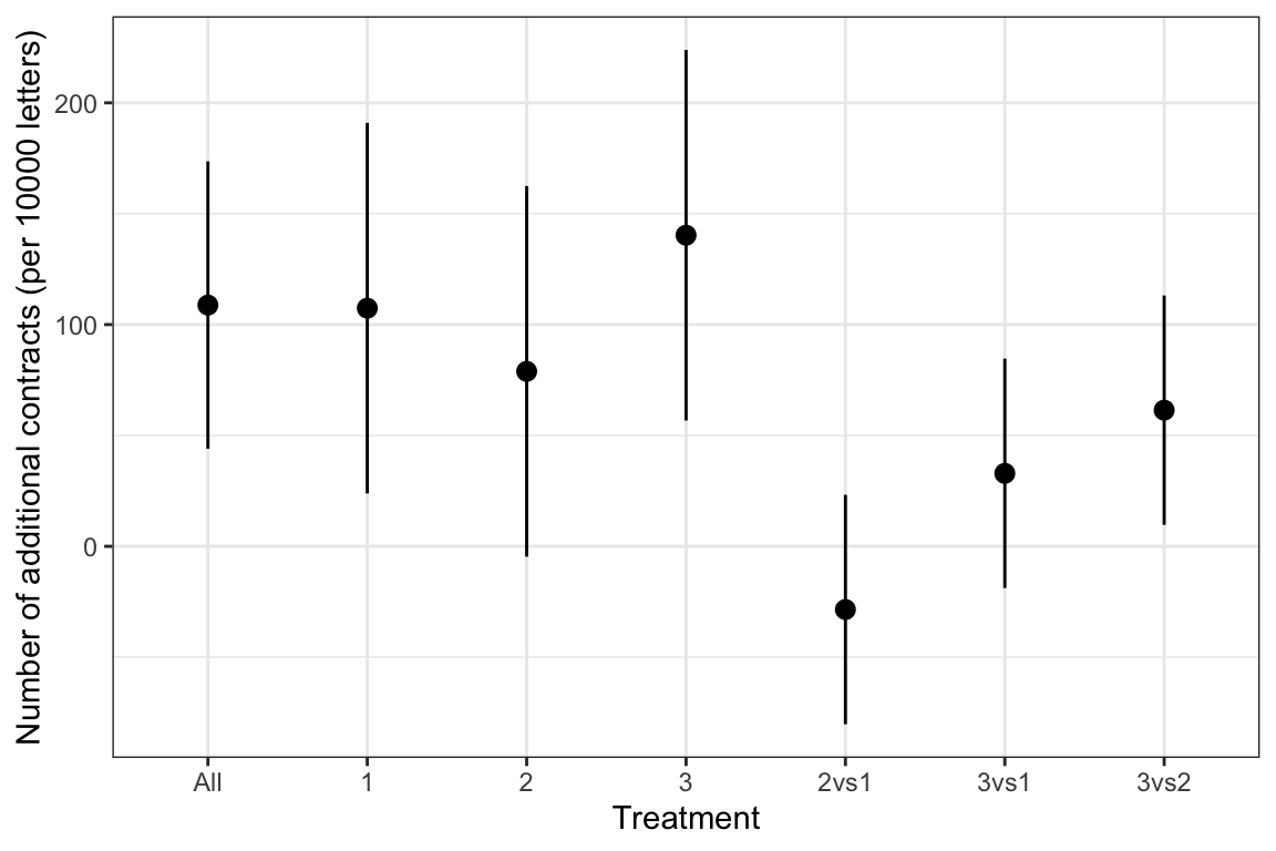
- Sending letters increases the number of contract applications by 109 \(\pm\) 66 per 10000 letters, a doubling of the baseline uptake.
- Personalized letters with a handwritten phrase appealing to people’s empathetic tendencies toward environmental conservation – Treatment 3 – had the largest impact. The difference with the simple letter is 33 \(\pm\) 52 additional contracts per 10000 letters, a difference that is not statistically different from zero.
- When the same nudge was photocopied (Treatment 2), it performed worse than both treatment 3 (-61 \(\pm\) 52) and Treatment 1 (-28 \(\pm\) 52).
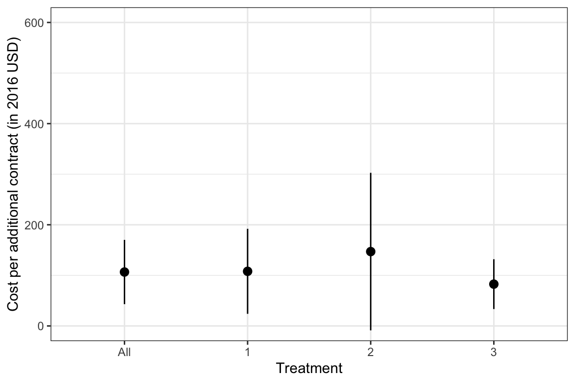
- The cost of an additional application is 107 \(\pm\) 64 2016USD.
Here is how we extracted the results from the paper.
Estimated treatment effects and their precision
Estimated treatment effects
Table 1 in the paper reports the proportion of farmers enrolling into the CSP (submitting an application file) under the control and treatment conditions (in percent):
- Control (no letter): \(1.009\),
- Treatment 1 (standard letter): \(2.083\)
- Treatment 2 (photocopied empathy nudge): \(1.798\)
- Treatment 3 (handwritten empathy nudge): \(2.412\)
- All treatments combined: \(2.097\)
Thanks to these numbers, we can build estimates of the treatment effects of each treatent (in percentage points). Let’s do that:
# enrollment rates (in percent)
czap.mean <- c(1.009,2.083,1.798,2.412,2.097)
names(czap.mean) <- c("Control","1","2","3","All")
# treatment effects vs control
czap.TE <- czap.mean[2:5]-czap.mean[[1]]
# treatment effects between treatments
czap.TE[5:6] <- czap.mean[3:4]-czap.mean[[2]]
czap.TE[7] <- czap.mean[4]-czap.mean[[3]]
names(czap.TE)[5:7] <- c("2vs1","3vs1","3vs2")
Precision of treatment effects
One difficulty that we have is that Czap et al (2019) do not provide standard errors. They do provide \(p-\)values though and we are going to try to use these as a way to back out precision. The \(p-\)value of the mean difference between any of the treatment conditions vs the control group is smaller than \(0.001\). It is also the case for each of the three independent treatments taken in isolation. The differences between treatment conditions are all non significantly different from zero, except the one between Treatment 2 and Treatment 3, which has a \(p-\)value of \(0.02\). We are going to invert these \(p-\)values and to apply the resulting precision estimate to the other comparisons between treatments.
# function for inverting p-values
se.pval <- function(pval,beta){
  return(beta/qnorm(1-pval/2))
}

# pvalues
czap.pval <- c(0.001,0.001,0.001,0.001,0.02,0.02,0.02)
names(czap.pval) <- names(czap.TE)

# computing precision
czap.se <- rep(0,length(czap.pval))
names(czap.se) <- names(czap.TE)
# for treatment against control
czap.se[1:4] <- purrr::map2_dbl(czap.pval[1:4],czap.TE[1:4],se.pval)
# we replace the individual treatment estimates of precision by the least precise one
czap.se[1:2] <- czap.se[[3]]

# for treatment 3 against 2
czap.se[7] <- purrr::map2_dbl(czap.pval[7],czap.TE[7],se.pval)
# we replace the individual treatment estimates of precision by the last one
czap.se[5:6] <- czap.se[[7]]

# putting results together in a dataframe
czap <- as.data.frame(cbind(czap.TE,czap.se))
colnames(czap) <- c('TE','SeTE')
czap$Treatment <- rownames(czap)
Cost-effectiveness of each treatment
Czap et al (2019) report a cost per letter of \(c=1.16\) 2016USD. That means that cost-effectiveness can be estimated by dividing \(c\) by the treatment effect (or additional number of contracts per letter): \(\hat{CE}=\frac{c}{\hat\beta}\). The standard error of the cost effectiveness can be obtained by the delta method: \(\hat\sigma_{CE}=\frac{c}{\hat\beta^2}\hat\sigma_{\beta}\). Let us now compute these terms for the two samples.
# function for computing standard error of cost-effectiveness
se.CE <- function(beta,sigmabeta,c=1.16){
  return(sigmabeta*c/(beta^2))
}

# generate cost-effectiveness
c <- 1.16 # cost per letter in dollars 2012
czap <- czap %>%
          mutate(
            TE = TE*100, # all effects per 10000 letters
            SeTE = SeTE*100,# all effects per 10000 letters
            CE = c*10000/TE,# cost of 10000 letters divided by number of contracts
            SeCE = map2_dbl(TE,SeTE,se.CE,c=c*10000) #standard error
          )
Sending results to SKAI
We are now ready to send our results to SKAI.
# reading connection informations
source(here::here("idSQL.R"))
# connecting to SQL server
HdF <- dbConnect(MySQL(), dbname="HdF",
                     user=myid, password=mypass, host=myhost)
# sending Results table
dbWriteTable(HdF,"czap",czap,overwrite=TRUE)
# commenting the table
dbSendQuery(HdF,"ALTER TABLE `HdF`.`czap`
    CHANGE COLUMN `TE` `TE` DOUBLE NULL DEFAULT NULL COMMENT 'The effect of the treatment measured as an increase in contract applications per 10000 farmers.' ,
    CHANGE COLUMN `SeTE` `SeTE` DOUBLE NULL DEFAULT NULL COMMENT 'The standard error of the estimated treatment effect.' ,
    CHANGE COLUMN `Treatment` `Treatment` TEXT NULL DEFAULT NULL COMMENT 'The treatment analysed.\nAll refers to all the treatments combined.\nTreatment 1: standard letter with the usual focus on the financial incentives offered by the program administrators. \nTreatment 2: photocopied empathy nudge. The language related to empathy nudging included: ''In the last two years, over 1600 of your fellow Nebraska farmers joined the common cause and enrolled/re-enrolled into the Conservation Stewardship Program.'' and ''Consider our role as caretakers of our natural resources, on which we depend on for our survival. Consider the impact of your decisions on wildlife habitat, water and air quality, your local community, and future generations.'' ''Join your fellow Nebraska farmers and ranchers in protecting our land!'' was added at the bottom of the letter next to the signature. The mention was written by the state conservationist and photocopied on every letter sent in the treatment 2 condition.\nTreatment 3: same as treatment 2 except that the empathy nudge was handwritten by research assistants.' ,
    CHANGE COLUMN `CE` `CE` DOUBLE NULL DEFAULT NULL COMMENT 'Cost-effectiveness of the treatment, in 2016 dollars by additional contract.',
    CHANGE COLUMN `SeCE` `SeCE` DOUBLE NULL DEFAULT NULL COMMENT 'Standards error of the cost-effectiveness of the treatment, in 2016 dollars by additional contract.',
    COMMENT = 'Table containing the estimated treatment effects of the letters sent to nudge farmers to subscribe Payments for Environmental Services in the CSP experiment of Czap et al (2019).' ;
")
# disconnecting the connection to the SQL server
dbDisconnect(HdF)