Testing and correcting for publication bias
The basic approach follows Kvarven et al (2019): we confront the results of meta-analysis and of methods to correct for publication bias to the results of pre-registered replications. To ensure that the meta-analysis are not influenced by the results of the replications, we only consider meta-analysis published before the replications took place. As in Kvarven et al (2019), we use 15 effects measured in psychology, for which we have both the original estimated effect size, results from a meta-analysis and from a pre-registered replication. We use the pre-registration estimate as the true benchmark and we compare it to the original estimate, the meta-analytic estimate and the estimates of various methods correcting for publication bias.
Empirical assessment of funnel plots
The first order of business is to try to build a very quick bird’s eye view of the extent and shape of selection bias in the 15 datasets used by Kvarven et al (2019). They have all been downloaded from the OSC repository of the Kvarven paper into a separate MySQL server, so that all calls to the datasets are normalized. Let’s first download the datasets.
## On Mac, this is the way to read files
source(here::here("idsql.R"))
kvarven <- dbConnect(MySQL(), dbname="Kvarven",
                     group='LaLonde_amazon',
                     user=myid, password=mypass, host=myhost)
# list of datasets
names.datasets <- dbGetQuery(kvarven,"SELECT `TABLE_NAME` FROM `information_schema`.`COLUMNS` WHERE (`TABLE_SCHEMA` = 'Kvarven');") %>%
                    pull(TABLE_NAME) %>%
                    unique()
# dowload data
fromSQL <- names.datasets %>% map(~dbReadTable(kvarven, .)) %>% set_names(names.datasets) # returns a list with as many elements as datasets for this paper_id
# disconnect from server
dbDisconnect(kvarven)
Now, for each dataset, we want to plot the funnel plot along with the replication-based estimate of the true effect size. One way to do that is to regroup all datasets into one and to use the facetwrap function of ggplot. But first, we have to define a new variable taking as value the name of the dataset, which will be our grouping variable in the facets. Let’s see how we can do that.
Studies <- fromSQL[2:16] # Omit the first table: it is the aggregated table, containing the summary of the results of each meta-analysis and each replication
# function generating a new column in a dataframe whose value is unique and in a vector
NewColumnFun <- function(name,data){
  data <- data %>%
            mutate(
              Study = name
            )
  return(data)
}

# New list of datasets
Studies <- map2(names.datasets[-1],Studies,NewColumnFun)
names(Studies) <- names(fromSQL[-1])

# one dataset with all studies
DataFull <- Studies %>%
              bind_rows()
I also have to prepare the aggregated dataset to extract the name of the meta-analysis and the original study.
Aggregate <- fromSQL[[1]] %>%
              mutate(
                Study = str_split_fixed(metaanalysis," ",n=2),
                Original = str_split_fixed(original," ",n=2)#,
#                Replication = str_split(replication," ",n=2)
              )

Aggregate[["Study"]] <- Aggregate[["Study"]][,1]
Aggregate[["Original"]] <- Aggregate[["Original"]][,1]
#Aggregate[["Replication"]][is.na(Aggregate[["Replication"]])] <- "NA"
#Aggregate[["Replication"]][dim(Aggregate[["Replication"]])>1] <- Aggregate[["Replication"]][,1]

# Adding the name of the original study in the full dataset
DataFull <- DataFull %>%
              left_join(select(Aggregate,Study,Original),by="Study")
Let’s now plot the data.
ggplot(DataFull,aes(x=sed,y=d)) +
  geom_point()+
  geom_hline(data=Aggregate,aes(yintercept=replication_s,linetype='Replication'),color='blue') +
  geom_hline(data=Aggregate,aes(yintercept=meta_s,linetype='Meta-analysis'),color='green') +
  geom_hline(data=Aggregate,aes(yintercept=effecto,linetype='Original'),color='red') +
  coord_cartesian(ylim=c(-1,2))+
  facet_wrap(~Original)+
  theme_bw()+
  xlab('Standard error of effect size')+
  ylab('Effect size') +
  scale_linetype_manual(name="Estimate",values=c(2,3,2),guide = guide_legend(override.aes = list(color = c("green", "red", "blue"))))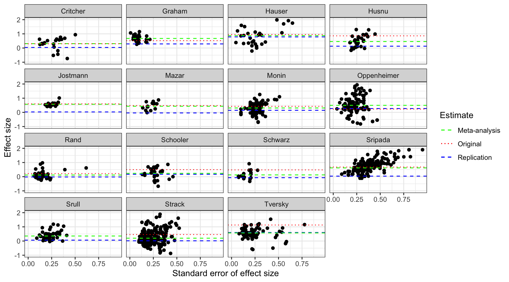
Funnel plot of the studies in Kvarven et al
The plot shows a very regular pattern over studies: the original effect is most of the time larger than the meta-analytic effect (while it is some time of the same magnitude) and the replication effect is generally smaller than the meta-analytic effect. Now the key question is whether these patterns could have been detected and predicted by a method correcting for publication bias.
PEESE
The first method we are going to try is the PEESE method proposed by Stanley and Doucouliagos. There are several ways to implement the method (with fixed or random effects, using a Funnel Asymmetry Test and Precision Effect Test before using the PEESE). Here, we are going to start with the simplest approach: use PEESE alone using a Weighted Least Squares estimator as advocated recently by Stanley and Doucouliagos (2015). The Weighted Least Squares estimator uses a fixed effect estimator for the main effect (and should thus be less sensitive to publication bias) but also reflects uncertainty due to treatment effect heterogeneity in its standard errors). We will use FAT-PET-PEESE later.
The first thing to do is to generate the weights for the WLS estimator.
# Generating weights for WLS
DataFull <- DataFull %>%
  group_by(Study) %>%
  mutate(
    vard =sed^2,
    weights = (1 / vard)/(sum(1 / vard))
  )
Now, let us run the PEESE WLS estimator for each meta-analytic study and recover the intercept, which is the estimated impact corrected for publication bias. We can also recover the coefficient on the variance of the treatment effect, so as to be able to represent the PEESE adjustments on the plot.
# Running the PEESE regressions and taking the results back
PEESE <- do(DataFull,tidy(lm(d ~ vard,weights=weights,data=. )))

# sending the PEESE estimates to the Aggregate dataset
Aggregate <- Aggregate %>%
              left_join(select(filter(PEESE,term=="(Intercept)"),Study,estimate,std.error),by="Study") %>%
              rename(
                PEESE_estimate= estimate,
                PEESE_estimate_se = std.error
                ) %>%
              left_join(select(filter(PEESE,term=="vard"),Study,estimate,std.error),by="Study") %>%
              rename(
                PEESE_var_estimate= estimate,
                PEESE_var_estimate_se = std.error
                )
Let us now plot the resulting PEESE estimates:
Let’s now plot the data. One thing that seems important and nice is the ability to visualize the PEESE curve. That is going to require some work in R.
# generating the data for plotting the PEESE curves
# function for generating the PEESE curve
PEESE_fun <- function(a,b){
  return(a+b*2^2)
}
# grid of points for sed
grid.sed <- seq(0,1,0.1)
# drawing the PEESE curves by iterating over the values of the two parameters
PEESE_curves <- map2(Aggregate$PEESE_estimate, Aggregate$PEESE_var_estimate, ~ .x + .y*grid.sed^2) %>%
  set_names(Aggregate$Original) %>%
  bind_cols(.)
# append to grid to the dataset
PEESE_curves$grid <- grid.sed
# pivot the dataset in long format to use with facet_wrap
PEESE_curves <- PEESE_curves %>%
                  pivot_longer(!grid,names_to="Original",values_to="PEESE_pred")
Let us plot the resulting estimates
ggplot(DataFull,aes(x=sed,y=d)) +
  geom_point()+
  geom_hline(data=Aggregate,aes(yintercept=replication_s,linetype='Replication'),color='blue') +
  geom_hline(data=Aggregate,aes(yintercept=meta_s,linetype='Meta-analysis'),color='green') +
  geom_hline(data=Aggregate,aes(yintercept=effecto,linetype='Original'),color='red') +
  geom_line(data=PEESE_curves,aes(x=grid,y=PEESE_pred,linetype='PEESE'),color='black') +
  coord_cartesian(ylim=c(-1,2))+
  facet_wrap(~Original)+
  theme_bw()+
  xlab('Standard error of effect size')+
  ylab('Effect size') +
  scale_linetype_manual(name="Estimate",values=c(2,3,2,2),guide = guide_legend(override.aes = list(color = c("green", "red","black", "blue"))))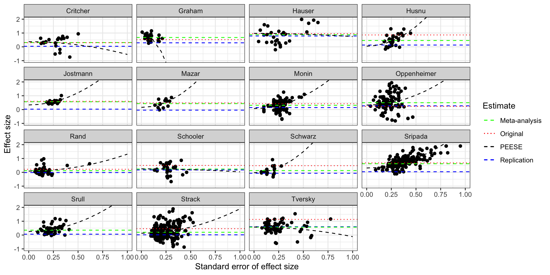
Funnel plot of the studies in Kvarven et al with PEESE
The plot shows the how the PEESE estimator works: it fits a quadratic curve through the data and its bias-corrected estimate is the intercept of this curve. For the Graham dataset, PEESE interprets wrongly the increase in effect size with precision as signaling that publication bias was coming from above (censoring of imprecise large results) and pushes the estimate above the meta-analytic one, further away from the truth. For the Crichter and Hauser datasets, PEESE makes the same mistake but the consequences are much less severe, and PEESE ends up very close to the meta-analytic estimate. There is one case in which PEESE works badly For all the other datasets, PEESE is closer to the truth than the meta-analytic estimate. The PEESE correction is sometimes spectacular, like in the Husnu, Monin, Oppenheimer and Schwarz datasets, where PEESE is indistiguishable from the true effect.
Most of the action on the graph occurs for low values of the replicated effect size. There, the original estimates are much more biased than the meta-analytic ones, which are themselves more biased than PEESE. PEESE does badly in the intermediate range of replication effect sizes because of the overestimated effect in the Graham study. A version of the estimator that would not implement any correction when the correlation between effect size and its standard error is negative would avoid similar mistakes and would work better than PEESE.
FAT-PET-PEESE
The classical approach proposed by Stanley and Doucouliagos is to implement the FAT-PET-PEESE estimator.
Their approach is based on three steps:
- The Funnel Asymmetry Test (FAT) tests whether there is a relationship between effect sizes and their precision. FAT uses as its null the hypothesis that the value of the slope in a regression of effect sizes on their precision measured by their standard error is zero. If there is no sign of publication bias, keep the estimate from the normal meta-analysis. If there is sign of publication bias, move to step 2.
- The Precision-Effect Test (PET) estimates the effect corrected for publication bias and tests for its existence. PET uses as its null the hypothesis that the value of the constant in a regression of effect sizes on their precision measured by their standard error is zero. If the null is not rejected, the assumed value of the meta-analytic treatment effect is zero (or at least the constant? it is the only way to get a standard error (we are going to try both)). If the null is rejected, move to step 3.
- The Precision-Effect Estimate with Standard Error (PEESE) estimates the effect corrected for publication bias using a non-linear model for the standard error. When there is a genuine effect, PEESE offers a less biased estimate than PET.
The first thing we need is to code a function that will spit out the FAT-PET-PEESE estimator for a given dataset.
# computing the FAT-PET-PEESE function
# it is a function of:
# data: dataset on which the tests are performed
# FAT.alpha: value of the size of the FAT test
# FAT.oneside: if TRUE, performs a one-sided FAT test, otherwise two-sided.
# PET.alpha: value of the size of the PET test
# PET.oneside: if TRUE, performs a one-sided PET test, otherwise two-sided.
# FAT.neg: if TRUE, discard FATPETPEESE estimates when the slope of the FAT test is negative
fatpetpeese <- function(data,FAT.alpha=0.05,FAT.oneside=FALSE,PET.alpha=0.05,PET.oneside=FALSE,FAT.neg=TRUE){
  # WLS meta-analysis
  wls.reg <- lm(d ~ 1,weights=weights,data=data)
  wls.est <- coefficients(wls.reg)[[1]]
  wls.est.se <- sqrt(vcov(wls.reg)[1,1])
  # FAT and PET regression
  fat.pet.reg <- lm(d ~ sed,weights=weights,data=data)
  fat.pet.est <- coefficients(fat.pet.reg)[[1]]
  fat.pet.est.se <- sqrt(vcov(fat.pet.reg)[1,1])
  fat.pet.slope <- coefficients(fat.pet.reg)[[2]]
  fat.pet.slope.se <- sqrt(vcov(fat.pet.reg)[2,2])
  # PEESE regression
  peese.reg <- lm(d ~ vard,weights=weights,data=data)
  peese.est <- coefficients(peese.reg)[[1]]
  peese.est.se <- sqrt(vcov(peese.reg)[1,1])
  peese.slope <- coefficients(peese.reg)[[2]]
  peese.slope.se <- sqrt(vcov(peese.reg)[2,2])
  # FAT test: t-test of assumption that slope is zero with FAT.alpha size (no correction for degrees of freedom)
  # value one for evidence of publication bias, zero otherwise
  if (FAT.oneside==TRUE){
    fat.test <- if_else(fat.pet.slope/fat.pet.slope.se>qnorm(1-FAT.alpha),1,0) # value one for evidence of publication bias, zero otherwise
  }
  if (FAT.oneside==FALSE){
    fat.test <- if_else(abs(fat.pet.slope/fat.pet.slope.se)>qnorm(1-FAT.alpha/2),1,0)
  }
  # if no signs of publication bias, go back to WLS meta-analytic estimate
  if (fat.test==0){
   fat.pet.peese.est <- wls.est
   fat.pet.peese.est.se <- wls.est.se
  }
  # if signs of publication bias, test whether the PET effect is different from zero or not
  # if not different from zero, keep zero as an estimate (for now, maybe we'll keep the PET estimate at some point)
  if (fat.test==1){
    # PET test: t-test of assumption that constant is zero with 5% size (no correction for degrees of freedom)
    if (PET.oneside==TRUE){
      pet.test <- if_else(coefficients(fat.pet.reg)[[1]]/(sqrt(vcov(fat.pet.reg)[1,1]))>qnorm(1-PET.alpha),1,0) # value one for evidence of effect, zero otherwise
    }
    if (PET.oneside==FALSE){
      pet.test <- if_else(abs(coefficients(fat.pet.reg)[[1]]/(sqrt(vcov(fat.pet.reg)[1,1])))>qnorm(1-PET.alpha/2),1,0) # value one for evidence of effect, zero otherwise
    }
    # if no sign of effect, we put zero in the estimated effect (and keep the PET standard error) (we could use the WLS or the PEESE one here, but that does not matter much)
    if (pet.test==0){
      fat.pet.peese.est <- 0
      fat.pet.peese.est.se <- sqrt(vcov(fat.pet.reg)[1,1])
    }
    # if there is evidence of effect, we run the PEESE estimator
    if (pet.test==1){
      # we keep the peese estimates as our main estimates
      fat.pet.peese.est <- peese.est
      fat.pet.peese.est.se <- peese.est.se
    }
  }
  # if FAT.neg=TRUE, we discard the FAT PET PEESE results in favor of the WLS results if the FAT slope is negative
  if (FAT.neg==TRUE){
    if (sign(fat.pet.slope)==-1){
      fat.pet.peese.est <- wls.est
      fat.pet.peese.est.se <- wls.est.se
    }
  }
  results <- as.data.frame(t(c(fat.pet.peese.est,fat.pet.peese.est.se,wls.est,wls.est.se,fat.pet.est,fat.pet.est.se,fat.pet.slope,fat.pet.slope.se,peese.est,peese.est.se,peese.slope,peese.slope.se)))
  colnames(results) <- c("FATPETPEESE.effect","FATPETPEESE.effect.se","WLS.effect","WLS.effect.se","FATPET.effect","FATPET.effect.se","FATPET.slope","FATPET.slope.se","PEESE.effect","PEESE.effect.se","PEESE.slope","PEESE.slope.se")
  return(results)
}
Let us now try to run FAT-PET-PEESE regression on all our datasets.
# trying the fatpetpeese function
test <- fatpetpeese(data=filter(DataFull,Study=="Belle"),FAT.oneside = TRUE,FAT.alpha = 0.1,FAT.neg=FALSE)

# Running the FAT_PET_PEESE regressions and taking the results back
FATPETPEESE <- do(DataFull,fatpetpeese(data=.,FAT.oneside = TRUE,FAT.alpha = 0.1,FAT.neg=TRUE))

# sending the PEESE estimates to the Aggregate dataset
Aggregate <- Aggregate %>%
              left_join(FATPETPEESE,by="Study")
Let us build the PEESE and the FAT curves.
# generating the data for plotting the PEESE curves and the FATPET
# grid of points for sed
grid.sed <- seq(0,1,0.1)
# drawing the FAT curves by iterating over the values of the two parameters
FATPET_curves <- map2(Aggregate$FATPET.effect, Aggregate$FATPET.slope, ~ .x + .y*grid.sed) %>%
  set_names(Aggregate$Original) %>%
  bind_cols(.)
# append to grid to the dataset
FATPET_curves$grid <- grid.sed
# pivot the dataset in long format to use with facet_wrap
FATPET_curves <- FATPET_curves %>%
                  pivot_longer(!grid,names_to="Original",values_to="FATPET_pred")

# drawing the PEESE curves by iterating over the values of the two parameters
PEESE_curves <- map2(Aggregate$PEESE.effect, Aggregate$PEESE.slope, ~ .x + .y*grid.sed^2) %>%
  set_names(Aggregate$Original) %>%
  bind_cols(.)
# append to grid to the dataset
PEESE_curves$grid <- grid.sed
# pivot the dataset in long format to use with facet_wrap
PEESE_curves <- PEESE_curves %>%
                  pivot_longer(!grid,names_to="Original",values_to="PEESE_pred")
Let’s see what it looks like:
# generating the data for plotting the PEESE curves
ggplot(DataFull,aes(x=sed,y=d)) +
  geom_point()+
  geom_hline(data=Aggregate,aes(yintercept=replication_s,linetype='Replication'),color='blue') +
  geom_hline(data=Aggregate,aes(yintercept=meta_s,linetype='Meta-analysis'),color='green') +
  geom_hline(data=Aggregate,aes(yintercept=WLS.effect,linetype='WLS'),color='purple') +
  geom_hline(data=Aggregate,aes(yintercept=effecto,linetype='Original'),color='red') +
  geom_line(data=PEESE_curves,aes(x=grid,y=PEESE_pred,linetype='PEESE'),color='black') +
  geom_line(data=FATPET_curves,aes(x=grid,y=FATPET_pred,linetype='FATPET'),color='black') +
  geom_hline(data=Aggregate,aes(yintercept=FATPETPEESE.effect,linetype='FATPETPEESE'),color='black') +
  coord_cartesian(ylim=c(-1,2))+
  facet_wrap(~Original)+
  theme_bw()+
  xlab('Standard error of effect size')+
  ylab('Effect size') +
  scale_linetype_manual(name="Estimate",values=c(2,3,2,3,2,2,3),guide = guide_legend(override.aes = list(color = c("black","black","green", "red","black", "blue","purple"))))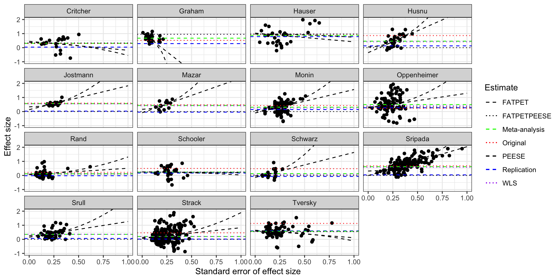
Funnel plot of the studies in Kvarven et al with PEESE and FATPETPEESE
Actually, I should replace the PEESE estimate with the WLS meta-analytic estimate. I also should use the WLS meta-analytic estimate as my main estimate and not the original one from Kvarven, since their estimation procedure is unclear and might involve random effects estimation, which magnifies publication bias. TO DO
FAT-PET-PEESE without the negative correlations
What if instead of computing the PEESE estimate when the correlation between effect size and standard error is negative, we were simply keeping the initial meta-analytic estimate? This is exceedingly simple to do. We just replace the PEESE estimate by the original meta-analytic estimate when the coefficient on the variance of the treatment effect is negative. Let’s just do it.
# computing the PEESE positive estimates
Aggregate <- Aggregate %>%
              mutate(PEESEpos_estimate = if_else(PEESE_var_estimate>0,PEESE_estimate,WLS.effect))
What would all zeroes look like?
p-curving
p-curving has been proposed by Uri Simonsohn, Leif Nelson and Joseph Simmons. It is extensively described in my book Statistical Tools for Causal Inference. p-curving was initially proposed as a way to test for the existence of p-hacking using an excess mass of p-values close to 0.05. The same set of authors has also proposed to use p-curving to correct for publication bias. This approach is also extensively described in Statistical Tools for Causal Inference. The idea of p-curving is to make use of the fact that the distribution of statistically significant p-values is uniform under the true distribution. This distribution is called the pp-curve, and the p-curving estimator chooses the value of the true treatment effect that minimizes the distance between the empirical pp-curve and a uniform. Let’s use the code provided in STCI in order to run this estimator on our datasets.
# Computation of one pp-value for true parameter value thetac and a list of estimates thetak with standard error sigmak
ppCurveEst <- function(thetac,thetak,sigmak,alpha=0.05){
  return((pnorm((thetac-thetak)/sigmak)/pnorm(thetac/sigmak-qnorm(1-alpha/2))))
}
#KS statistic
KS.stat.unif <- function(vector){
  return(ks.test(x=vector,y=punif)$statistic)
}
# Distance between the p-curve and the uniform, for a given true value thetac
ppCurve.Loss.KS <- function(thetac,thetak,sigmak,alpha=0.05){
  ppvalues <- ppCurveEst(thetac=thetac,thetak=thetak,sigmak=sigmak,alpha=alpha)
  return(KS.stat.unif(ppvalues))
}
#Estimating thetac that minimizes the KS distance by brute grid search first
# will program the optimize function after
# thetak vector of (statistically significant) estimates
# sigmak vector of standard errors of (statistically significant) estimates
# thetacl and thetach: upper and lower bounds of the grid search
# ngrid: number of grid points
ppCurveEstES <- function(thetak,sigmak,thetacl,thetach,alpha=0.05,ngrid=100){
  # break thetac values in a grid
  thetac.grid <- seq(from=thetacl,to=thetach,length.out=ngrid)
  # computes the ppcurve for each point of the grid: outputs a matrix where columns are the ppcurves at each values of thetac
  ppCurve.grid <- sapply(thetac.grid,ppCurveEst,thetak=thetak,sigmak=sigmak,alpha=alpha)
  # compute KS stat for each value of thetac (over columns)
  KS.grid <- apply(ppCurve.grid,2,KS.stat.unif)
  # computes the value of thetac for which the KS stat is minimum (match identifies the rank of the min in the KSgrid)
  min.theta.c <- thetac.grid[match(min(KS.grid),KS.grid)]
  # optimizes over KS stat to find value of thetac that minimizes the KS stat
  thetahat <- optimize(ppCurve.Loss.KS,c(min.theta.c-0.1,min.theta.c+0.1),thetak=thetak,sigmak=sigmak,alpha=alpha)
  # returns the optimal thetac, the grid of thetac, the KS stats on the grid, for potential plot, and the ecdf of ppvalues at the optimum theta for graph against the uniform
  return(list(thetahat$minimum,thetac.grid,KS.grid,ecdf(ppCurve.grid[,match(min(KS.grid),KS.grid)])))
}

# Function adapted to data frames and variable names
ppCurveEstESVec <- function(data,theta,sigma,...){
  result <- ppCurveEstES(thetak=pull(filter(data,data[,theta]>0,abs(data[,theta]/data[,sigma])>=qnorm((1+0.95)/2)),!!sym(theta)),pull(filter(data,data[,theta]>0,abs(data[,theta]/data[,sigma])>=qnorm((1+0.95)/2)),!!sym(sigma)),...)
  # returns the optimal thetac, the grid of thetac, the KS stats on the grid, for potential plot, and the ecdf of ppvalues at the optimum theta for graph against the uniform
  return(as.data.frame(result[[1]]))
}

# Function adapted to fitering by dataset
ppCurveEstESVecData <- function(DataName,data,...){
  result <- ppCurveEstESVec(data=filter(data,Study==DataName),...)
  return(result)
}
Let’s implement the functions:
# list of studies
studies <- DataFull %>% group_by(Study) %>% summarize(tot = n()) %>% pull(Study)
ppCurveTest <- ppCurveEstESVecData("Belle",data=DataFull,theta='d',sigma='sed',thetacl=0,thetach=1,alpha=0.05,ngrid=100)
# lapply to list of studies
ppCurve <- sapply(studies,ppCurveEstESVecData,data=DataFull,theta='d',sigma='sed',thetacl=0,thetach=1,alpha=0.05,ngrid=100)
ppCurve <- data.frame(ppCurve = unlist(ppCurve),Study = studies)
# merge with aggregate dataset
Aggregate <- Aggregate %>%
              left_join(ppCurve,by=c('Study'))
Let us now see what it looks like on the data:
# generating the data for plotting the PEESE curves
ggplot(DataFull,aes(x=sed,y=d)) +
  geom_point()+
  geom_hline(data=Aggregate,aes(yintercept=replication_s,linetype='Replication'),color='blue') +
  geom_hline(data=Aggregate,aes(yintercept=meta_s,linetype='Meta-analysis'),color='green') +
  geom_hline(data=Aggregate,aes(yintercept=WLS.effect,linetype='WLS'),color='purple') +
  geom_hline(data=Aggregate,aes(yintercept=effecto,linetype='Original'),color='red') +
  geom_hline(data=Aggregate,aes(yintercept=ppCurve,linetype='ppCurve'),color='black') +
  coord_cartesian(ylim=c(-1,2))+
  facet_wrap(~Original)+
  theme_bw()+
  xlab('Standard error of effect size')+
  ylab('Effect size') +
  scale_linetype_manual(name="Estimate",values=c(2,3,2,2,3),guide = guide_legend(override.aes = list(color = c("green", "red","black", "blue","purple"))))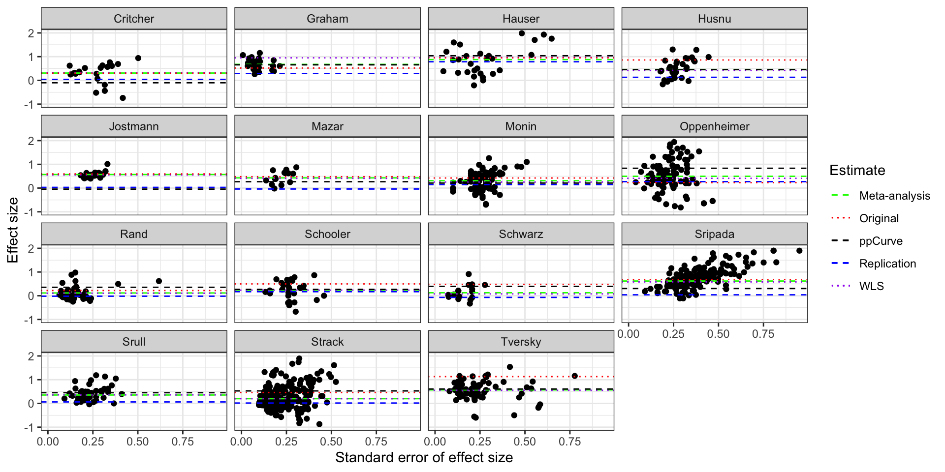
Funnel plot of the studies in Kvarven et al with ppCurve estimates
Selection models
Selection models model the joint distribution of treatment effects and of selection into publication as a way to correct for publication bias. The most recent installment of selection models is Andrews ans Kasy’s estimator. Let’s assume for now that the distribution of treatment effects is a normal. We might relax this assumption later. Let’s write the selection model:
# log-likelihood
Lk <- function(thetak,sigmak,p1,thetac,tau){
  f <- ifelse(thetak/sigmak<qnorm(1-0.05/2),p1,1)*dnorm((thetak-thetac)/sqrt(sigmak^2+tau^2))/(1-pnorm((qnorm(1-0.05/2)*sigmak-thetac)/sqrt(sigmak^2+tau^2))*(1-p1))
  return(sum(log(f)))
}
#log-likelihood prepared for nlminb: vector of parameters and minimization
Lk.param <- function(param,thetak,sigmak){
  f <- Lk(thetak=thetak,sigmak=sigmak,p1=param[[1]],thetac=param[[2]],tau=param[[3]])
  return(-f)
}

# Function adapted to data frames and variable names
Optim.Lk.param.Vec <- function(data,thetak,sigmak,...){
  optim.Lk <- stats::nlminb(objective=Lk.param,thetak=pull(data,!!sym(thetak)),sigmak=pull(data,!!sym(sigmak)),...)
  paramAK <- rbind(optim.Lk$par)
  colnames(paramAK) <- c("$p_1$","$\\theta_c$","$\\tau$")
  return(paramAK)
}

# Function adapted to fitering by dataset
Optim.Lk.param.Vec.Data <- function(DataName,data,...){
  result <- Optim.Lk.param.Vec(data=filter(data,Study==DataName),...)
  return(result)
}
Let’s now run the estimation for all of our datasets:
# optimization procedure using nlminb
MaxEval<-10^5
MaxIter<-10^5
Tol<-10^(-8)
stepsize<-10^(-6)
# I force a fixed effects meta-analysis by setting tau2=0
lower.b <- c(0,-Inf,0)
upper.b <- c(1,Inf,0)
start.val <- c(0.5,1,0)

# test with Belle
optim.Lk.Belle <- Optim.Lk.param.Vec.Data(DataName="Belle",data=DataFull,thetak="d",sigmak="sed",start=start.val,lower=lower.b,upper=upper.b,control=list(eval.max=MaxEval,iter.max=MaxIter,abs.tol=Tol))
# lapply to list of studies
SelModel <- t(sapply(studies,Optim.Lk.param.Vec.Data,data=DataFull,thetak="d",sigmak="sed",start=start.val,lower=lower.b,upper=upper.b,control=list(eval.max=MaxEval,iter.max=MaxIter,abs.tol=Tol)))
colnames(SelModel) <- c("p1","SelModel","tau")
SelModel <- as.data.frame(SelModel)
SelModel$Study <- studies
# merge with aggregate dataset
Aggregate <- Aggregate %>%
              left_join(select(SelModel,Study,SelModel),by=c('Study'))
Let us now see what it looks like on the data:
# generating the data for plotting the PEESE curves
ggplot(DataFull,aes(x=sed,y=d)) +
  geom_point()+
  geom_hline(data=Aggregate,aes(yintercept=replication_s,linetype='Replication'),color='blue') +
  geom_hline(data=Aggregate,aes(yintercept=meta_s,linetype='Meta-analysis'),color='green') +
  geom_hline(data=Aggregate,aes(yintercept=WLS.effect,linetype='WLS'),color='purple') +
  geom_hline(data=Aggregate,aes(yintercept=effecto,linetype='Original'),color='red') +
  geom_hline(data=Aggregate,aes(yintercept=SelModel,linetype='Selection Model'),color='black') +
  coord_cartesian(ylim=c(-1,2))+
  facet_wrap(~Original)+
  theme_bw()+
  xlab('Standard error of effect size')+
  ylab('Effect size') +
  scale_linetype_manual(name="Estimate",values=c(2,3,2,2,3),guide = guide_legend(override.aes = list(color = c("green", "red", "blue","black","purple"))))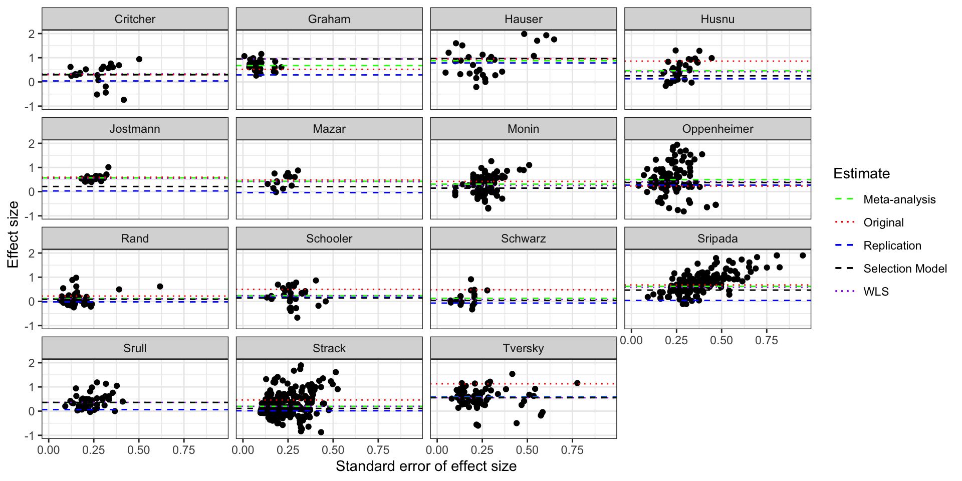
Funnel plot of the studies in Kvarven et al with Selection Model estimates
Regularizing estimates by their mean bias
Performance of the estimators
One way to compute the performance of the PEESE estimator (or of any estimator) is to report some statistics for its distance to the truth (taken here to be the replication estimate). Let us compute several such estimates: the mean bias, the mean absolute deviation and the root mean squared error. We will do that for the PEESE estimator and for the meta-analytic estimator, in order to measure the improvement in estimation brought about by the PEESE estimator over the meta-analytic estimate.
# computing the bias of each estimator
Aggregate <- Aggregate %>%
                mutate(
                  PEESE_bias = PEESE_estimate-replication_s,
                  PEESEpos_bias = PEESEpos_estimate-replication_s,
                  FATPETPEESEpos_bias = FATPETPEESE.effect-replication_s,
                  ppCurve_bias = ppCurve-replication_s,
                  SelModel_bias = SelModel-replication_s,
                  Meta_bias = WLS.effect-replication_s,
                  Original_bias = effecto-replication_s
                  )
# Computing the mean absolute deviation and root mean square error of each estimator
Estim_bias <- Aggregate %>%
                summarize(
                  PEESE_MeanBias = mean(PEESE_bias),
                  PEESE_MAD = mean(abs(PEESE_bias)),
                  PEESE_RMSE = sqrt(mean(PEESE_bias^2)),
                  PEESEpos_MeanBias = mean(PEESEpos_bias),
                  PEESEpos_MAD = mean(abs(PEESEpos_bias)),
                  PEESEpos_RMSE = sqrt(mean(PEESEpos_bias^2)),
                  FATPETPEESEpos_MeanBias = mean(FATPETPEESEpos_bias),
                  FATPETPEESEpos_MAD = mean(abs(FATPETPEESEpos_bias)),
                  FATPETPEESEpos_RMSE = sqrt(mean(FATPETPEESEpos_bias^2)),
                  ppCurve_MeanBias = mean(ppCurve_bias),
                  ppCurve_MAD = mean(abs(ppCurve_bias)),
                  ppCurve_RMSE = sqrt(mean(ppCurve_bias^2)),
                  SelModel_MeanBias = mean(SelModel_bias),
                  SelModel_MAD = mean(abs(SelModel_bias)),
                  SelModel_RMSE = sqrt(mean(SelModel_bias^2)),
                  Meta_MAD = mean(abs(Meta_bias)),
                  Meta_MeanBias = mean(Meta_bias),
                  Meta_RMSE = sqrt(mean(Meta_bias^2)),
                  Original_MeanBias = mean(Original_bias),
                  Original_MAD = mean(abs(Original_bias)),
                  Original_RMSE = sqrt(mean(Original_bias^2))
                )
We are going to send these estimates to a table on SKY and we will use them to generate a graph of the performances of various methods for correcting for publication bias at the top of this page.
# putting the estimates in long format
Method_bias <- Estim_bias %>%
                pivot_longer(
                  cols=1:ncol(Estim_bias),
                  names_to=c("Method","Value"),
                  names_sep= "_",
                  values_to = "value"
                ) %>%
                pivot_wider(
                  id_cols=Method,
                  names_from=Value
                )

# sending the estimates to SKY
# connecting
source(here::here("idsql.R"))
SKY <- dbConnect(MySQL(), dbname="SKY",
                     user=myid, password=mypass, host=myhost)
# sending
dbWriteTable(SKY,"Correct_Pub_Bias",Method_bias,overwrite=TRUE)
# disconnecting
dbDisconnect(SKY)
Finally, a very useful way to visualize our results is to plot the original, meta-analytic and PEESE estimates against the truth.
# preparing dataset for the plot: pivoting longer
plotXYdata <- Aggregate %>%
                select(Original,replication_s,effecto,WLS.effect,PEESE_estimate,PEESEpos_estimate,FATPETPEESE.effect) %>%
                pivot_longer(
                  cols=effecto:FATPETPEESE.effect,
                  names_to="Method",
                  values_to="Estimate"
                ) %>%
                rename(
                  Replication = replication_s
                ) %>%
                mutate(
                  Method = if_else(Method=="effecto","Original",
                                   if_else(Method=="WLS.effect","Meta-analysis",
                                           if_else(Method=="PEESE_estimate","PEESE",
                                                   if_else(Method=="FATPETPEESE.effect","FATPETPEESEpos","PEESEpos")))),
                  Method=factor(Method,levels=c("Original","Meta-analysis","PEESE","PEESEpos","FATPETPEESEpos"))
                )

# plot
ggplot(plotXYdata,aes(x=Replication,y=Estimate,color=Method)) +
  geom_point()+
  geom_smooth(se = FALSE)+
  geom_function(fun=~.x,color="black",linetype="dashed")+
  coord_cartesian(xlim=c(-0.1,0.8),ylim=c(-0.1,3))+
  theme_bw() +
  xlab("Replication effect size") +
  ylab("Estimated effect size")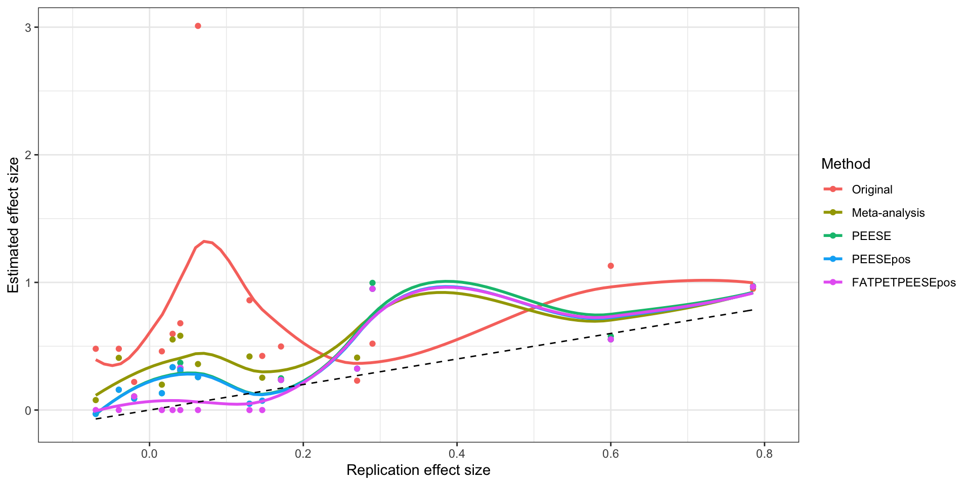
Original, meta-analytic and PEESE estimates as a function of the replication effect size
Another useful way to look at the data is to make a plot of the bias of each method with respect to the true effect size, and of the bias of the corrected estimates as a function of the bias in the original data or in the meta-analysis.
Bias with respect to the true effect size
Let us first build the bias of each method with respect to the true effect size.
# preparing dataset for the plot: pivoting longer
plotBiasXYdata <- Aggregate %>%
                select(replication_s,contains("_bias")) %>%
                pivot_longer(
                  cols=PEESE_bias:Original_bias,
                  names_to=c("Method","Suppl"),
                  values_to="Bias",
                  names_sep='_'
                ) %>%
                select(-Suppl) %>%
                rename(
                  Replication = replication_s
                ) %>%
                mutate(
                  Method=factor(Method,levels=c("Original","Meta","PEESE","PEESEpos","FATPETPEESEpos","SelModel","ppCurve"))
                )

# plot
ggplot(plotBiasXYdata,aes(x=Replication,y=Bias,color=Method)) +
  geom_point()+
  geom_smooth(se = FALSE)+
#  geom_function(fun=~.x,color="black",linetype="dashed")+
#  coord_cartesian(xlim=c(-0.1,0.8),ylim=c(-0.1,3))+
  theme_bw() +
  xlab("Replication effect size") +
  ylab("Bias")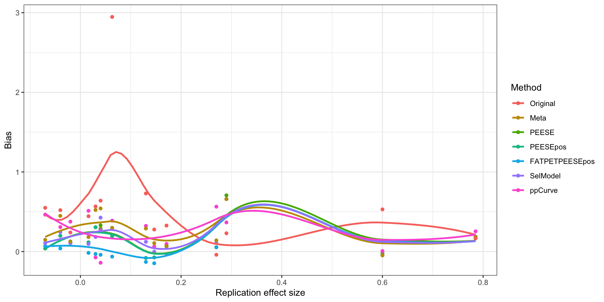
Bias of estimates as a function of the replication effect size
Bias with respect to initial bias
Let us now plot the bias of each method with respect to the initial bias (the one with the original estimate or the meta-analysis).
Bias with respect to the original effect
# preparing dataset for the plot: pivoting longer
plotBiasOriginalXYdata <- Aggregate %>%
                select(contains("_bias")) %>%
                pivot_longer(
                  cols=PEESE_bias:Meta_bias,
                  names_to=c("Method","Suppl"),
                  values_to="Bias",
                  names_sep='_'
                ) %>%
                select(-Suppl) %>%
                mutate(
                  Method=factor(Method,levels=c("Meta","PEESE","PEESEpos","FATPETPEESEpos","SelModel","ppCurve"))
                )

# plot
ggplot(plotBiasOriginalXYdata,aes(x=Original_bias,y=Bias,color=Method)) +
  geom_point()+
  geom_smooth(se = FALSE)+
  geom_function(fun=~.x,color="black",linetype="dashed")+
  coord_cartesian(xlim=c(-0.1,1),ylim=c(-0.1,1))+
  theme_bw() +
  xlab("Bias of original estimate") +
  ylab("Bias")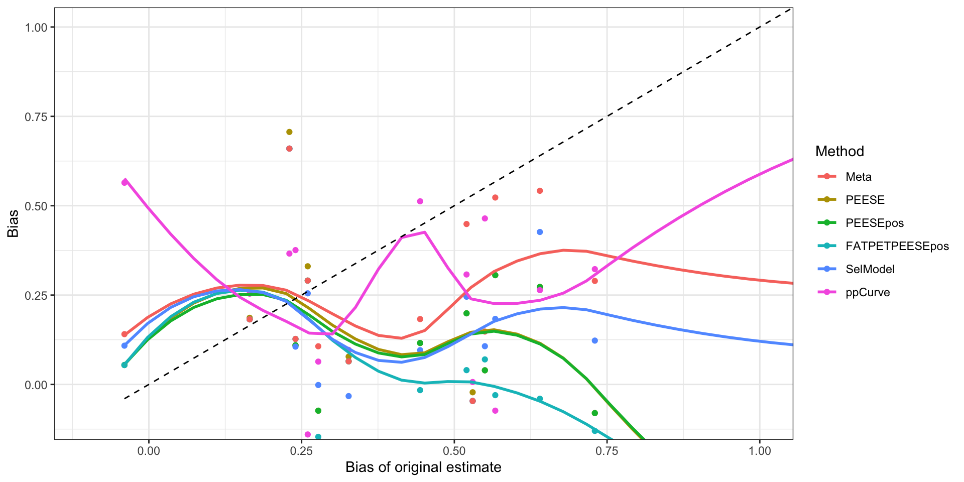
Bias of estimates as a function of the bias of the original estimate
Bias with respect to the meta-analytic estimate
# preparing dataset for the plot: pivoting longer
plotBiasMetaXYdata <- Aggregate %>%
                select(contains("_bias")) %>%
                pivot_longer(
                  cols=PEESE_bias:SelModel_bias,
                  names_to=c("Method","Suppl"),
                  values_to="Bias",
                  names_sep='_'
                ) %>%
                select(-Suppl) %>%
                mutate(
                  Method=factor(Method,levels=c("PEESE","PEESEpos","FATPETPEESEpos","SelModel","ppCurve"))
                )

# plot
ggplot(plotBiasMetaXYdata,aes(x=Original_bias,y=Bias,color=Method)) +
  geom_point()+
  geom_smooth(se = FALSE)+
  geom_function(fun=~.x,color="black",linetype="dashed")+
  coord_cartesian(xlim=c(-0.1,1),ylim=c(-0.1,1))+
  theme_bw() +
  xlab("Bias of meta-analytic estimate") +
  ylab("Bias")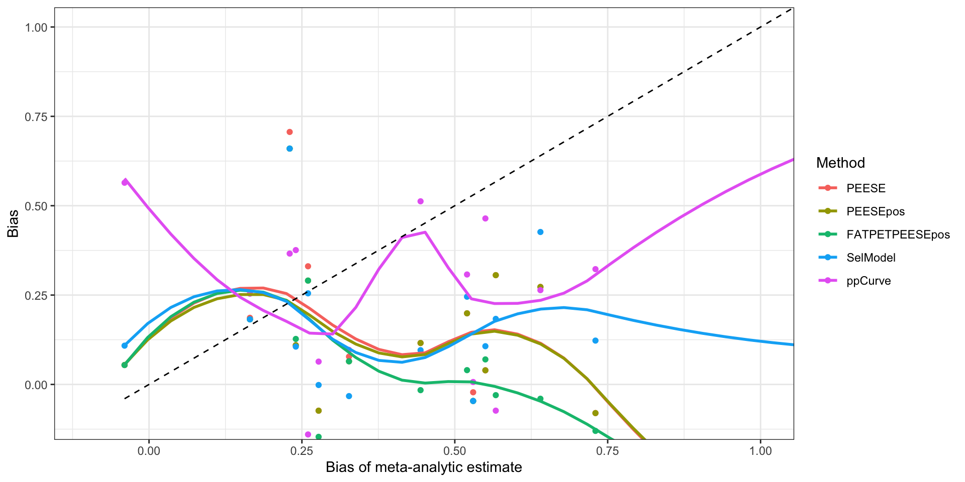
Bias of estimates as a function of the bias of the meta-analytic estimate
Run FATPETPEESE wuthout pos Run FATPET with and without pos, including the one forcing the zeroes (stopping just before PEESE) Run FATPETPEESE with alpha=0.05 for both tests